1.3 Example: Frierfjord macrofauna

The first example is from the IOC/GEEP practical workshop on biological effects of pollutants ( Bayne, Clarke & Gray (1988) ), held at the University of Oslo, August 1986. This attempted to contrast a range of biochemical, cellular, physiological and community analyses, applied to field samples from potentially contaminated and control sites, in a fjordic complex (Frierfjord/Langesundfjord) linked to Oslofjord ({F}, Fig. 1.1). For the benthic macrofaunal component of this study ( Gray, Aschan, Carr et al. (1994) ), four replicate 0.1m2 Day grab samples were taken at each of six sites (A-E and G, Fig 1.1) and, for each sample, organisms retained on a 1.0 mm sieve were identified and counted. Wet weights were determined for each species in each sample, by pooling individuals within species.

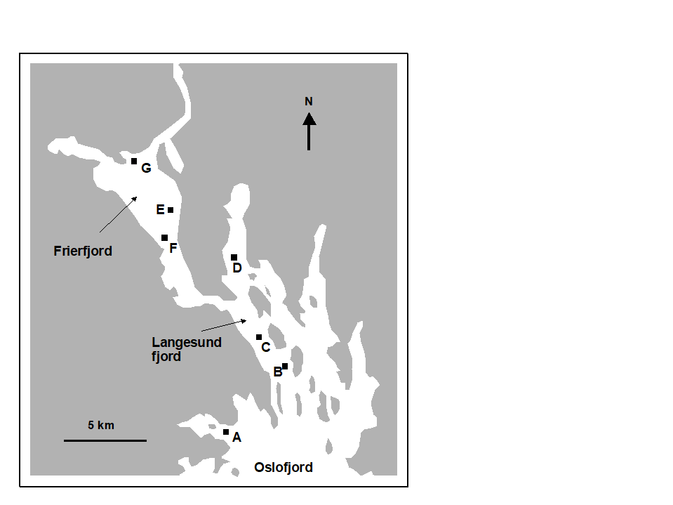Fig. 1.1. Frierfjord, Norway {F}. Benthic community sampling sites (A-G) for the IOC/GEEP Oslo Workshop; site F omitted for macrobenthos.

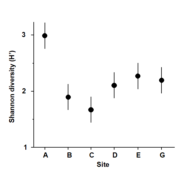
Fig. 1.2. Frierfjord macrofauna {F}. Means and 95% confidence intervals for Shannon diversity (H'), from four replicates at each of six sites (A-E, G).

Part of the resulting data matrix can be seen in Table 1.2: in total there were 110 different taxa categorised from the 24 samples. Such matrices (abundance, A, and/or biomass, B) are the starting point for the biotic analyses of this manual, and this example is typical in respect of the relatively high ratio of species to samples (always >> 1) and the prevalence of zeros. Here, as elsewhere, even an undesirable reduction to the 30 ‘most important’ species (see Chapter 2) leaves more than 50% of the matrix consisting of zeros. Standard multivariate normal analyses (e.g. Mardia, Kent & Bibby (1979) ) of these counts are clearly ruled out; they require both that the number of species (variables) be small in relation to the number of samples, and that the abundance or biomass values are transformable to approximate normality: neither is possible.

Table 1.2. Frierfjord macrofauna {F}. Abundance and biomass matrices (part only) for the 110 species in 24 samples (four replicates at each of six sites A-E, G); abundance in numbers per 0.1m2, biomass in mg per 0.1m2.

Species	Samples

	A1	A2	A3	A4	B1	B2	B3	B4
Abundance
Cerianthus lloydi	0	0	0	0	0	0	0	0
Halicryptus sp.	0	0	0	1	0	0	0	0
Onchnesoma	0	0	0	0	0	0	0	0
Phascolion strombi	0	0	0	1	0	0	1	0
Golfingia sp.	0	0	0	0	0	0	0	0
Holothuroidea	0	0	0	0	0	0	0	0
Nemertina, indet.	12	6	8	6	40	6	19	7
Polycaeta, indet.	5	0	0	0	0	0	1	0
Amaena trilobata	1	1	1	0	0	0	0	0
Amphicteis gunneri	0	0	0	0	4	0	0	0
Ampharetidae	0	0	0	0	1	0	0	0
Anaitides groenl.	0	0	0	1	1	0	0	0
Anaitides sp.	0	0	0	0	0	0	0	0
. . . .
Biomass
Cerianthus lloydi	0	0	0	0	0	0	0	0
Halicryptus sp.	0	0	0	26	0	0	0	0
Onchnesoma	0	0	0	0	0	0	0	0
Phascolion strombi	0	0	0	6	0	0	2	0
Golfingia sp.	0	0	0	0	0	0	0	0
Holothuroidea	0	0	0	0	0	0	0	0
Nemertina, indet.	1	41	391	1	5	1	2	1
Polycaeta, indet.	9	0	0	0	0	0	0	0
Amaena trilobata	144	14	234	0	0	0	0	0
Amphicteis gunneri	0	0	0	0	45	0	0	0
Ampharetidae	0	0	0	0	0	0	0	0
Anaitides groenl.	0	0	0	7	11	0	0	0
Anaitides sp.	0	0	0	0	0	0	0	0
. . . .

As discussed above, one easy route to simplification of this high-dimensional (multi-species) complexity is to reduce each matrix column (sample) to a single univariate description. Fig. 1.2 shows the results of computing the Shannon diversity (H', see Chapter 8) of each sample^¶, and plotting for each site the mean diversity and its 95% confidence interval, based on a pooled estimate of variance across all sites from the ANOVA table, Chapter 6. (An analysis of the type outlined in Chapter 9 shows that prior transformation of H' is not required; it already has approximately constant variance across the sites, a necessary prerequisite for standard ANOVA). The most obvious feature of Fig. 1.2 is the relatively higher diversity at the control/reference location, A.

---

^¶ Using the PRIMER DIVERSE routine.