4.4 PCA for environmental data
The above example makes it clear that PCA is an unsatisfactory ordination method for biological data. However, PCA is a much more useful in the multivariate analysis of environmental rather than species data¶. Here variables are perhaps a mix of physical parameters (grain size, salinity, water depth etc) and chemical contaminants (nutrients, PAHs etc). Patterns in environmental data across samples can be examined in an analogous way to species data, by multivariate ordination, and tools for linking biotic and environmental summaries are fully discussed in Chapter 11.
PCA is more appropriate to environmental variables because of the form of the data: there are no large blocks of zero counts; it is no longer necessary to select a dissimilarity coefficient which ignores joint absences, etc. and Euclidean distance thus makes more sense for abiotic data. However, a crucial difference between species and environmental data is that the latter will usually have a complete mix of measurement scales (salinity in ‰, grain size in $\phi$ units, depth in m, etc). In a multi-dimensional visualisation of environmental data, samples are points referred to environmental axes rather than species axes, but what does it mean now to talk about (Euclidean) distance between two sample points in the environmental variable space? If the units on each axis differ, and have no natural connection with each other, then point A can be made to appear closer to point B than point C, or closer to point C than point B, simply by a change of scale on one of the axes (e.g. measuring PCBs in $\mu$g/g not ng/g). Obviously it would be entirely wrong for the PCA ordination to vary with such arbitrary scale changes. There is one natural solution to this: carry out a correlation-based PCA, i.e. normalise all the variable axes (after transformations, if any) so that they have comparable, dimensionless scales.
The problem does not generally arise for species data, of course, because though a scale change might be made (e.g. from numbers of individuals per core to densities per m2 of sediment surface), the same scale change is made on each axis and the PCA ordination will be unaffected. If PCA is to be used for biotic as well as abiotic analysis, the default position would be to use correlation-based PCA for environmental data and covariance-based PCA for species data (but much better still, use an alternative ordination method such as MDS for species, starting from a more appropriate dissimilarity matrix, such as Bray-Curtis!). For both biotic or abiotic matrices, prior transformation is likely to be beneficial. Different transformations may be desirable for different variables in the abiotic analysis, e.g. contaminant concentrations will often be right-skewed (and require, say, a log transform) but salinity might be left-skewed and need a reverse log transform, see equation (11.2), or no transform at all. The transform issues are returned to in Chapter 9.
PCA strengths
-
PCA is conceptually simple. Whilst the algebraic basis of the PCA algorithm requires a facility with matrix algebra for its understanding, the geometric concepts of a best-fitting plane in the species space, and perpendicular projection of samples onto that plane, are relatively easily grasped. Some of the more recently proposed ordination methods, which either extend or supplant PCA (e.g. Principal Co-ordinates Analysis, Detrended Correspondence Analysis) can be harder to understand for practitioners without a mathematical background.
-
It is computationally straightforward, and thus fast in execution. Software is widely available to carry out the necessary eigenvalue extraction for PCA. Unlike the simplest cluster analysis methods, e.g. the group average UPGMA, which could be accomplished manually in the pre-computer era, the simplest ordination technique, PCA, has always realistically needed computer calculation. But on modern machines it can take small fractions of a second processing time for small to medium sized matrices. Computation time, however, will tend to scale with the number of variables, whereas with MDS, clustering etc, which are based on sample resemblances (and which have lost all knowledge of the species which generated these) computing time tends to scale with (squared) sample numbers.
-
Ordination axes are interpretable. The PC axes are simple linear combinations of the values for each variable, as in equation (4.1), so have good potential for interpretation, e.g. see the Garroch Head environmental data analysis in Chapter 11, Fig. 11.1 and equation (11.1). In fact, PCA is a tool best reserved for abiotic data and this Clyde data set is thus examined in much more detail in Chapter 11.
PCA weaknesses
-
There is little flexibility in defining dissimilarity. An ordination is essentially a technique for converting dissimilarities of community composition between samples into (Euclidean) distances between these samples in a 2- or higher-dimensional ordination plot. Implicitly, PCA defines dissimilarity between two samples as their Euclidean distance apart in the full p-dimensional species space; however, as has been emphasised, this is rather a poor way of defining sample dissimilarity: something like a Bray-Curtis coefficient would be preferred but standard PCA cannot accommodate this. The only flexibility it has is in transforming (and/or normalising) the species axes so that dissimilarity is defined as Euclidean distance on these new scales.
-
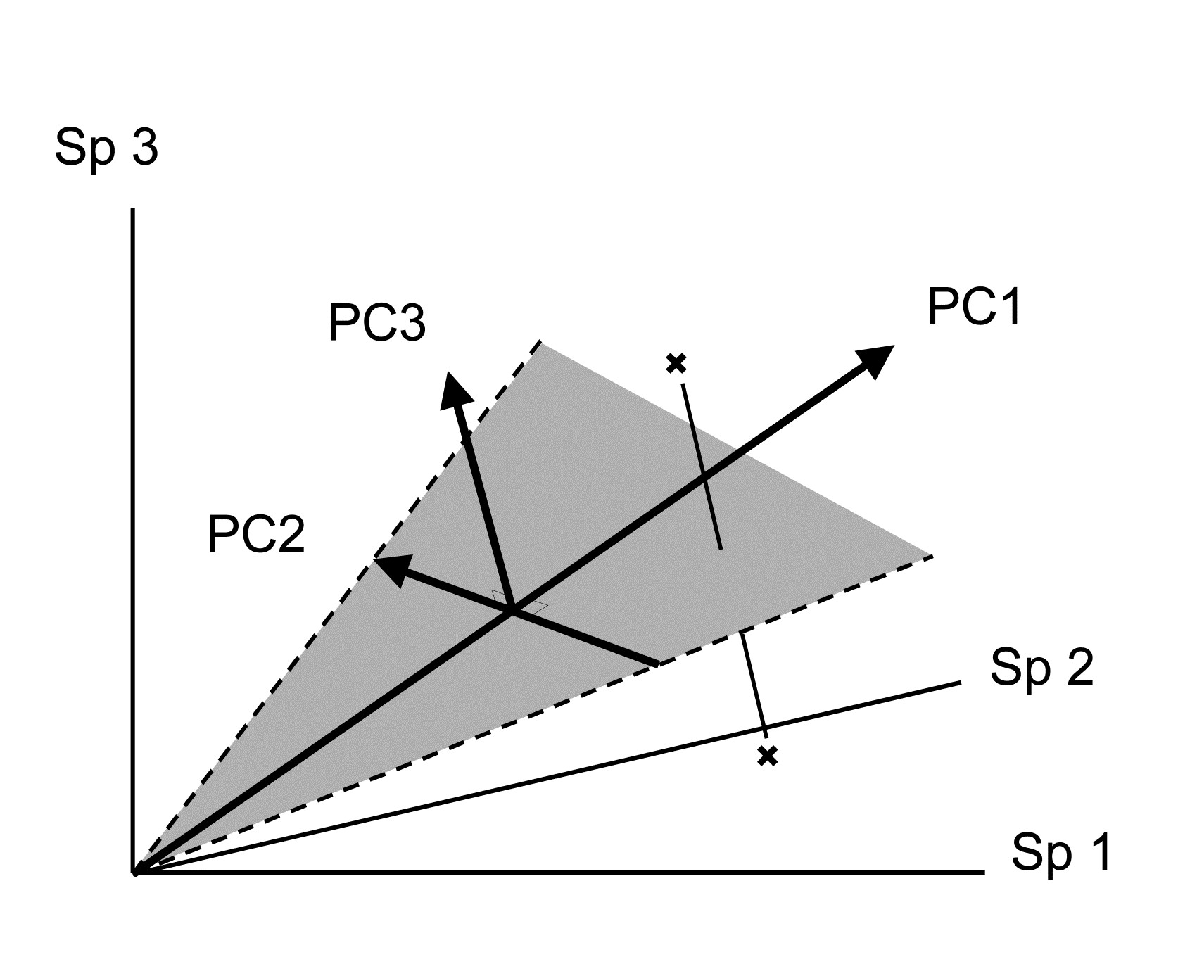
Its distance-preserving properties are poor. Having defined dissimilarity as distance in the p-dimensional species space, PCA converts these distances by projection of the samples onto the 2-dimensional ordination plane. This may distort some distances rather badly. Taking the usual visual analogy of a 2-dimensional ordination from three species, it can be seen that samples which are relatively far apart on the PC3 axis can end up being co-incident when projected (perhaps from ‘opposite sides’) onto the (PC1, PC2) plane.
¶ An environmental data matrix can be input to PRIMER in the same way as a species matrix, though it is helpful to identify its Data type as ‘Environmental’ (other choices are ‘Abundance’, ‘Biomass’ or ‘Other’) because PRIMER then offers sensible default options for each type, e.g. in the selection of Resemblance coefficient. In statistics texts, the data matrix is usually described as having n rows (samples) by p columns (variables) whereas the biological matrices we have seen so far have always had species variables as rows (the reason for this convention in biological contexts is clear: p is often larger than n, and binomial species names are much more neatly displayed as row than column labels!). It is not necessary to transpose either matrix type before entry into PRIMER: in the Open dialog, simply select whether the input matrix has samples as rows or columns, or amend that information later (on the Edit>Properties menu) if it has been incorrectly entered initially.