11.6 Linkage trees (and example)
The idea of linkage trees¶ is most easily understood in the context of a particular example, so Fig. 11.12 redisplays some of the nMDS bubble plots for the 17 Exe estuary sites used to illustrate the BEST/Bio-Env procedure, earlier in this chapter. Bio-Env shows that three variables, MPD, Sal% and H$_2$S, can ‘explain’ a large (and significant, Fig. 11.11) component of the multivariate biotic structure but this does not tell us how they explain the structure, e.g. for the five main clusters seen in Fig. 5.4, which abiotic variables are distinguishing which clusters? The answer is readily seen in this case from a few simple bubble plots, but this is only possible because the 2-d MDS stress is low (0.05) and thus the plot is reliable. In general it would be useful to have some means of describing how particular abiotic variables ‘explain’ particular divisions of samples in the full, high-d biotic space: the PRIMER LINKTREE routine can be helpful here.
Binary divisive clustering was introduced on page 3.6. The unconstrained clustering technique described there (UNCTREE) divides each sample set into two subsets, successively, each binary division being chosen in some optimum way, until a stopping rule is triggered, which is typically a SIMPROF test failing to demonstrate community differences among the remaining samples in a group. LINKTREE, in contrast, is a constrained binary divisive clustering, in which the only subdivisions allowed are those for which an ‘explanation’ exists in terms of a threshold on one of the environmental variables in a separately supplied abiotic matrix for a matching set of samples. For the Exe nematode data, the first stage is shown in Fig. 11.12: MPD, Sal% and H$_2$S are considered one at a time. For Median Particle Diameter, the ‘best’ split of the full set of samples into two groups is shown on the biotic MDS for all 19 sites (seen previously at Fig 11.6), corresponding to the threshold MPD<0.18 for sites 1-4, 7-9 (sites to the left of the dotted line) and MPD>0.21 for the remaining sites (to the right), Fig. 11.12a. The ‘best’ split is defined here as that which maximises the ANOSIM R statistic between the two groups formed†, as was the case for the unconstrained (UNCTREE) procedure, and it does not use the MDS plot in any way – thus ensuring that the procedure works in the true high-d space of the biota data.
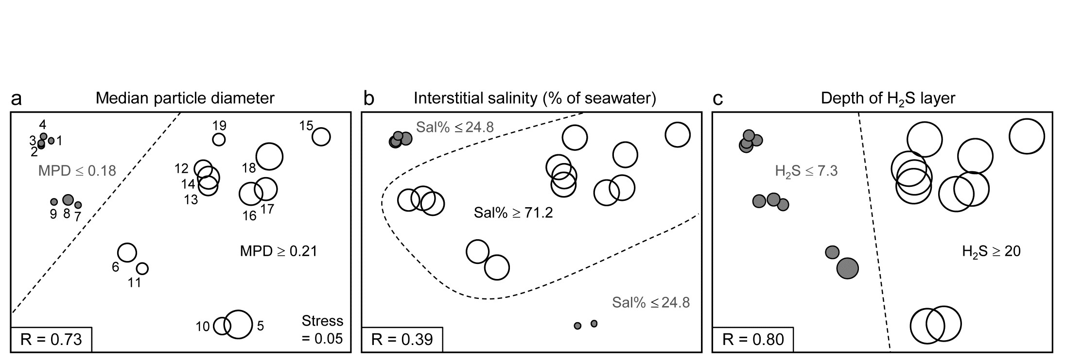
Fig. 11.12. Exe estuary nematodes {X}. First step in LINKTREE illustrated by a biotic nMDS of the 19 sites, as Fig. 11.6, with bubble plots for: a-c) median particle diameter, interstitial salinity (as % of 36ppt) and depth of the anoxic layer (cm). Dotted line indicates the optimal split of the communities at the 19 sites into two groups (open and closed circles), based on maximising the ANOSIM R statistic between them, subject to the constraint that the figured abiotic variable takes consistently lower values in one group than the other.
For LINKTREE (unlike UNCTREE), not all $2 ^ {18}$ ways of dividing 19 samples into two groups are permitted, because most of them will not correspond to a precise threshold on the median particle diameter. In fact, by ranking the sites in increasing MPD order, it is clear that we only need to consider 18 possible divisions in the constrained case (the site with smallest MPD vs. the rest, the two smallest vs. the rest, and so on). Fig. 11.2a shows the best of these 18 splits gives R=0.73.
Now the other two abiotic variables are considered in turn. Sal%, though important (as will be seen later), does not do a good job of an initial binary split, the best division giving only R=0.39 (Fig. 11.12b) – it is clear that sites are either of greatly reduced interstitial salinity (<24.8% of seawater) or are reasonably saline (>71.2%), with no sites in between. However, depth of the blackened H$_ 2$S layer separates the 19 sites into two groups best of all here, with R=0.80 (Fig 11.12c), so this becomes the first division (labelled A) in the dendrogram of Fig. 11.13a.
Each subset is now subject to further binary division, exploring thresholds on all three abiotic variables. It is clear from Fig. 11.12b, for example, that Sal% will provide the best explanation for the natural separation of sites (5,10) from (12-19), those for which H$_ 2$S>20 in the first split. This gives R=1, split G on Fig. 11.13a, and the remaining divisions proceed in the same way. The figure legend gives some detail on layout of the full divisive dendrogram of Fig. 11.3a. One point to note is that inequalities can be in either direction, e.g. the division at J has sites to the left with Sal%>89.4 and to the right with Sal%<89, and these will reverse if the dendrogram branches are arbitrarily rotated (in the same way as for any other dendrogram). Further, though all splits are shown§, it would be incorrect to interpret some, since they ‘fail’ the SIMPROF test, i.e. if there is no evidence of biological heterogeneity of samples in a current group, then there can be no justification for seeking an environmental explanation for further dividing that group – thus these parts of the dendrogram are ‘greyed out’.
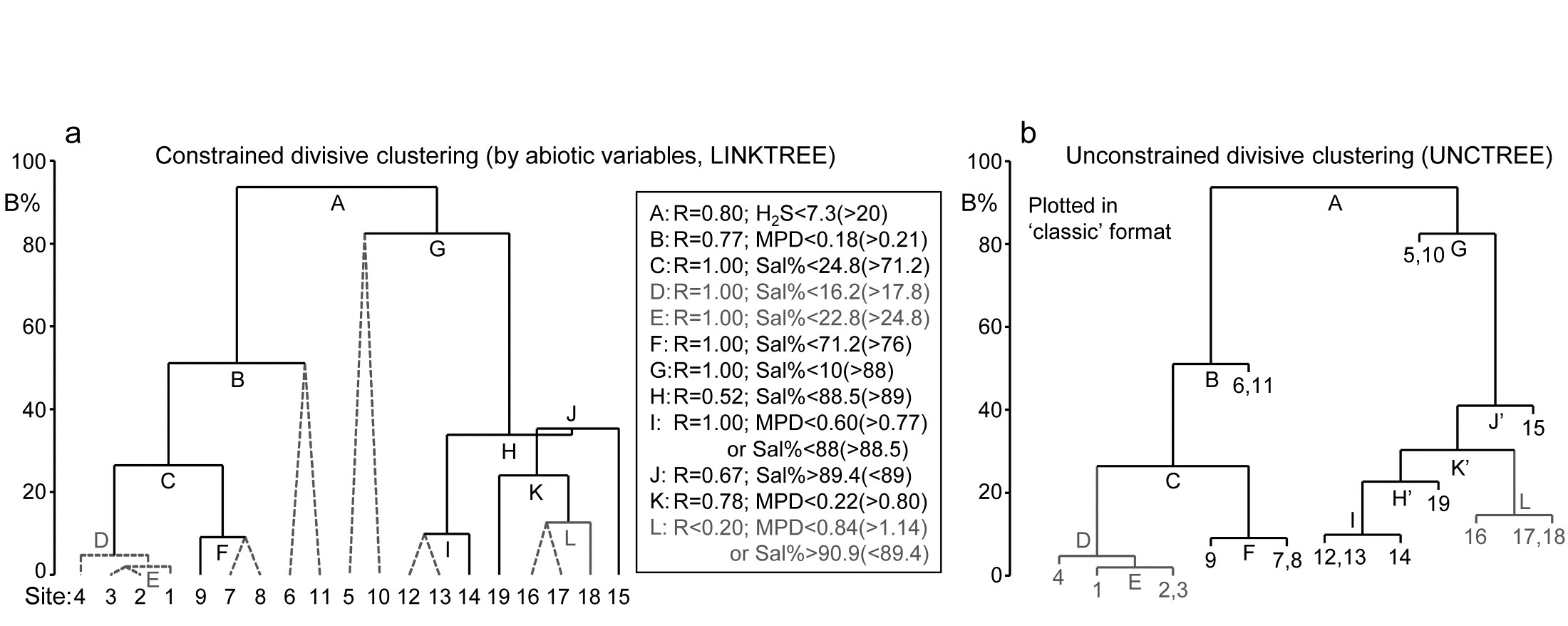
Fig. 11.13. Exe estuary nematodes {X}. a) Binary divisive clustering (LINKTREE) of the communities at 19 sites, for which step A was illustrated in Fig. 11.12, i.e. each split constrained by a threshold on one of the three abiotic variables: MPD, Sal%, H$_ 2$S. The first in-equality (e.g. for split A, H$_2$S<7.3) always indicates sites to the left side of the split, the second (in brackets, e.g. >20) sites to the right. The same splits will be obtained whether abiotic data is transformed or not (the process is truly non-parametric!) so the inequalities should always quote untransformed values, for greater clarity. Dotted or grey lines or text denote splits not to be interpreted because they are below the stopping rules; here the latter use SIMPROF tests before each split and also require that R>0.2 (e.g. the split at L would be allowed by SIMPROF but has R<0.2). The y axis scale (B%) is the average of the between-group rank dissimilarities, using the original ranks from the biotic resemblance matrix, scaled to take the value 100% if the first split is a perfect division (i.e. R=1).
b) Unconstrained binary divisive clustering (UNCTREE) of the same data, plotted in ‘classic’ style (e.g. as for LINKTREE in PRIMER v6; v7 allows both formats for either analysis). UNCTREE is based only on the biotic resemblances, with grey lines/letters again denoting divisions with R<0.2 or not supported by SIMPROF tests.
The scale on the y axis can be chosen (the A% scale) to make the divisions equi-step, arbitrarily, down the dendrogram (this is the option used in most standard CART programs) but here we display divisions at a y axis level (B%) which reflects the magnitude of differences between the subsets of samples formed at each division, in relation to the community structural differences across all samples. Such an absolute scale cannot be created from the ANOSIM R values used to make each split, since they continually ‘relativise’, by re-ranking the dissimilarities within each current set. Clarke, Somerfield & Gorley (2008) show that an appropriate scale can be based only on between-group average rank dissimilarity, using the original ranks from the full matrix. This is scaled by dividing by its value for the case of maximum possible separation of the first two groups produced by the initial division (the case R=1) and multiplying by 100, to give the B% scale. The Fig. 11.13a dendrogram does not quite start at B = 100 therefore, since the split seen in Fig. 11.12c gives R = 0.80 (clearly a few between group dissimilarities are smaller than some within group values) but the split at G is seen to be between very different groups (B = 82%), whilst that at, for example, D (the division of site 4 from 1 to 3), is inconsequential in comparison (B = 5%); that pattern is clear from the MDS plot.
An interesting but subtle point arises for split J, with its B = 35% value just exceeding that for H, a prior division (B = 34%). This reversal in the dendrogram is here an indication that the split of site 15 from (12-14, 16-19) would have been a more natural first step than the LINKTREE division of sites 12-14 from 15-19. In fact this is exactly what unconstrained (UNCTREE) clustering does, as seen in Fig. 11.13b (split J’). The point to note here is that LINKTREE is not able to make this more natural division because none of the three variables gives a threshold value which can separate site 15 from the set (12-14, 16-19). It is only after the group 12-14 has been removed that the separation of site 15 (now only from 16-19) has an ‘explanation’. So the presence of such reversals in a dendrogram could be an indication that an abiotic variable capable of ‘explaining’ a natural pattern has not been measured. Here, site 15 is discriminated by Ht (height up the shore) and, had that variable been included, the dendrogram would have separated 15 before others in that group. However, a reversal could equally well reflect large sampling variability in the biotic community or the measured abiotic variables – it is clear that LINKTREE is a technique suited only to robust data, with well-established detailed patterns in SIMPROF tests, and it is relevant that this successful example of a LINKTREE run is a case where both biotic and abiotic data have been (time-)averaged to reduce the variability‡.
One unwelcome result, however, of introducing more explanatory variables is that there are certain to be multiple explanations for each split, whereas this is only seen in a limited way in Fig. 11.13a, e.g. at split I, where a threshold on MPD or on Sal% will give the same division of sites (12,13) from 14. Had we used all 6 abiotic variables, nearly every division would have had multiple explanations, e.g. the first split A would have resulted from %Org>0.37(<0.24) as well as H$_ 2$S<7.3(>20). The routine can have no basis for choosing between ‘explanations’ which give the same split – neither may be causal, of course! So there is a strong incentive in LINKTREE to be disciplined and use few abiotic variables, chosen for their potential causality and likely independence, as now seen.
Example: Fal estuary nematodes
Fig. 11.14 shows the divisive LINKTREE clustering of 27 sites in 5 creeks of the Fal estuary, UK, based on nematode assemblages (creek map at Fig. 9.3, {f}). The creeks have varying levels of metal pollution by historic mining, here represented by sediment Cu concentrations (other metals being highly correlated with Cu), and a single grain size variable, %Silt/Clay.
Though the creek distinctions are not utilised at all, the resulting divisive clustering and SIMPROF tests largely divides the sites into their creeks (with a few sub-divisions), Fig. 11.14a. In spite of the non-trivial stress in this case (0.12), making the MDS (11.14b) only an approximation to the biotic relationships, it can be still be useful to indicate the sub-groupings, by increasingly fainter dividing lines, and the thresholds from the LINKTREE run, manually on the ordination.
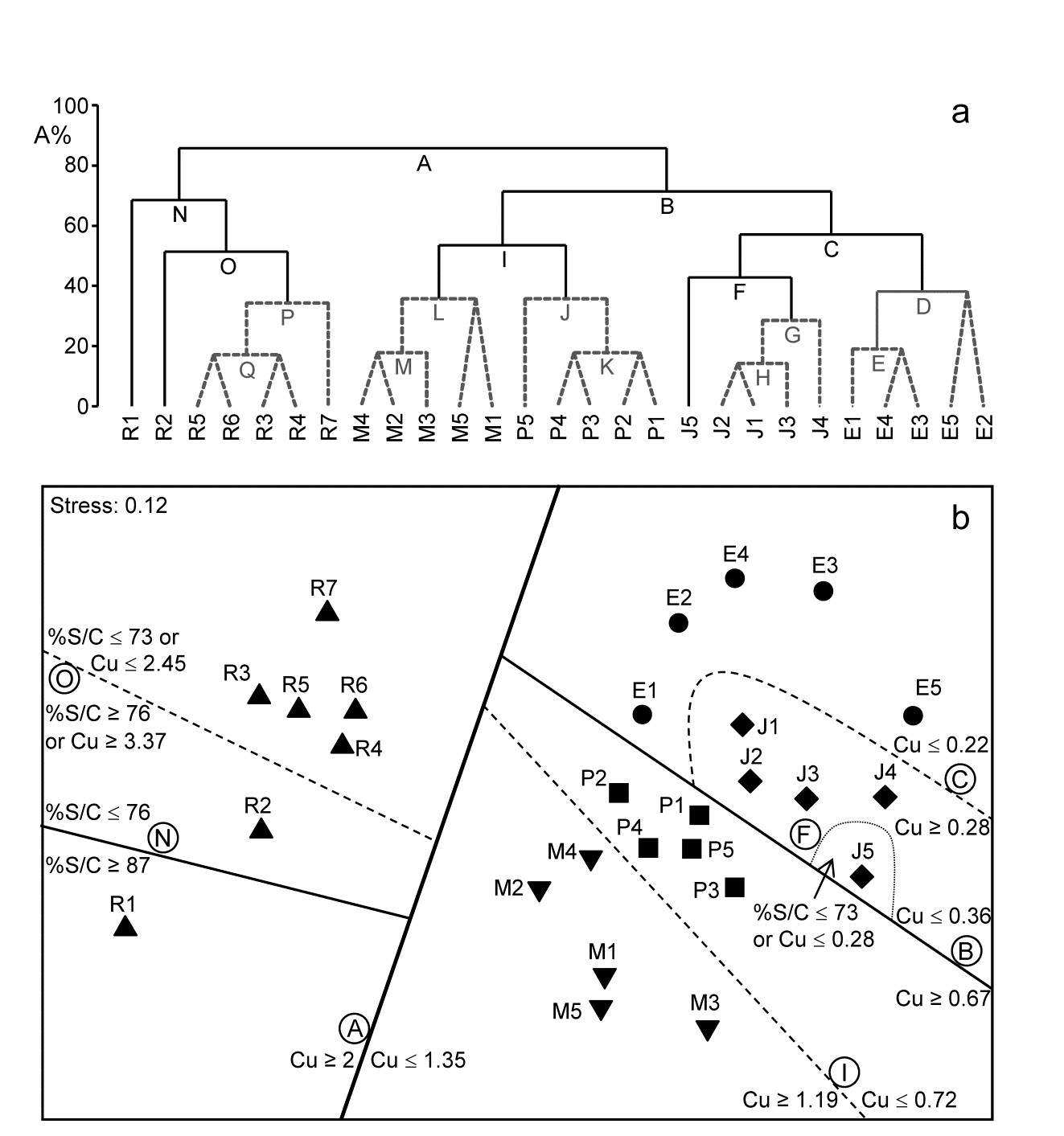
Fig. 11.14. Fal estuary nematodes {f}. a) Constrained divisive clustering (LINKTREE, using y axis scale A%, of arbitrary equi-steps), and b) nMDS of the 27 sites (in 5 creeks, see map in Fig. 9.3: Restronguet, Mylor, Pill, St Just, Percuil), based on fourth-root transformed counts and Bray-Curtis similarities. Divisions subject to thresholds on two environmental variables: sediment Cu concentration and %Silt/Clay ratio. Dashed lines and grey letters on the dendrogram denote groupings not supported by SIMPROF. Supported divisions identified by the same letters on the MDS, together with the inequalities ‘explaining’ them.
¶ De'Ath (2002) introduced this idea into ecology as ‘multivariate regression trees’, extending the ‘classification and regression trees’ (CART) routines found in major statistics packages such as S-Plus. Clarke, Somerfield & Gorley (2008) adapt this technique to be consistent with PRIMER’s non-parametric approach, and therefore use binary clustering divisions based on optimising the rank-based ANOSIM R statistic rather than, for example, maximising among- group sums of squares. They use the terminology ‘linkage trees’ since the method has little to do with model-based ‘regression’ as such (a historical term arising from the ‘regression to the mean’ seen when the slope of a linear relationship declines as the residual variance increases).
† As explained on page 3.6 we are not using ANOSIM as a test here, merely exploiting its very useful role as a measure of separation between groups of samples in multivariate space. Note therefore that the resemblance matrix among samples for each new set is re-ranked in order to calculate the R values for all the possible subsets from the next division. There are no constraints that subsets should be of comparable size. PRIMER does allow the user to debar groups of fewer than n samples (n specified) but there seems no good reason to rule out e.g. singleton groups, or not to split a group of less than n samples, if a SIMPROF test would allow it. (Note, however, that SIMPROF will never split a group of two samples, page 3.5). PRIMER can also allow a split not to be made if R does not exceed a threshold value – see later.
§ This is to make it possible to display labels or factor levels and symbols for the samples, rather than the previous LINKTREE format in PRIMER v6 (the ‘classic’ style of Fig. 11.13b) which was restricted to using sample numbers. In the new form, it can be incorporated into shade plots, see the sample axis in Fig. 7.8.
‡ LINKTREE can also sometimes succeed because of its total lack of assumptions and thus great flexibility. An (over)simple characterisation is that DISTLM (multivariate multiple linear regression in PERMANOVA+) assumes linearity and additivity of the abiotic variables on the high-d community response, whereas Bio-Env caters for non-linearity but still makes the additivity assumption, i.e. both are holistic methods applying across the full set of sites. For example, Ht (shore height) did not feature in Bio-Env results (Table 11.2) and would not do so in DISTLM, because its ‘effect’ is inconsistent across the sites: 1-4 have a wide range of shore heights yet identical communities (largely true of sites 7-9 also), whereas the assemblage at site 15 appears to be separated from all those at 12-19 by the greater shore height (the only variable that makes this split). If, as here, Ht only appears to be important to the community when the sediment is coarser (MPD>0.21), but does not matter at all when it is finer (MPD<0.18), Fig. 11.12a, this is exactly the definition of interaction (non-additivity) of the two abiotic variables in their effect on the biota. By the intuitive premise for Bio-Env (first paragraph on page 11.4 it is clear that the procedure will be ambivalent about including Ht in its explanation. Similarly, in modelled multiple regression, whilst DISTLM could theoretically be extended to include all interaction effects (in addition to all quadratic terms, to try to allow for the non-linear response) this is usually impossible because of the large number of model parameters that would then need fitting. LINKTREE is designed to cater for strong non-linearity through its use of thresholds, and interaction through its compartmentalisation – explanations are only local to a few sites not global. But it has major drawbacks: no allowance for sampling variability and an inability to cater sensibly for more than a few variables.