6.10 ANOSIM for ordered factors
Generalised ANOSIM statistic for the 1-way case
Now return to the simple one-way case of page 6.2, with multivariate data from a number of pre-specified groups (A, B, C, …, e.g. sites, times or treatments) and with replicate samples from each group. It is well known that the ANOSIM test, using the R statistic of equation 6.1, is formally equivalent to a non-parametric Mantel-type test (which PRIMER calls a RELATE test), in which the dissimilarities are correlated with a simple model matrix, using a Spearman rank correlation coefficient ($\rho$, introduced in equation 6.3). Such model matrices are idealised distance matrices which describe the structure expected under the alternative hypothesis (to the null hypothesis of ‘no differences between groups’), and a range of such models are introduced and discussed in Chapter 15, but here we need just the simple case in which samples in the same group are considered to be a distance 0 apart and in different groups a distance 1 unit apart. (The units are not important because Pearson correlation between matching elements is calculated having first ranked both matrices, which is the definition of a Spearman rank correlation).
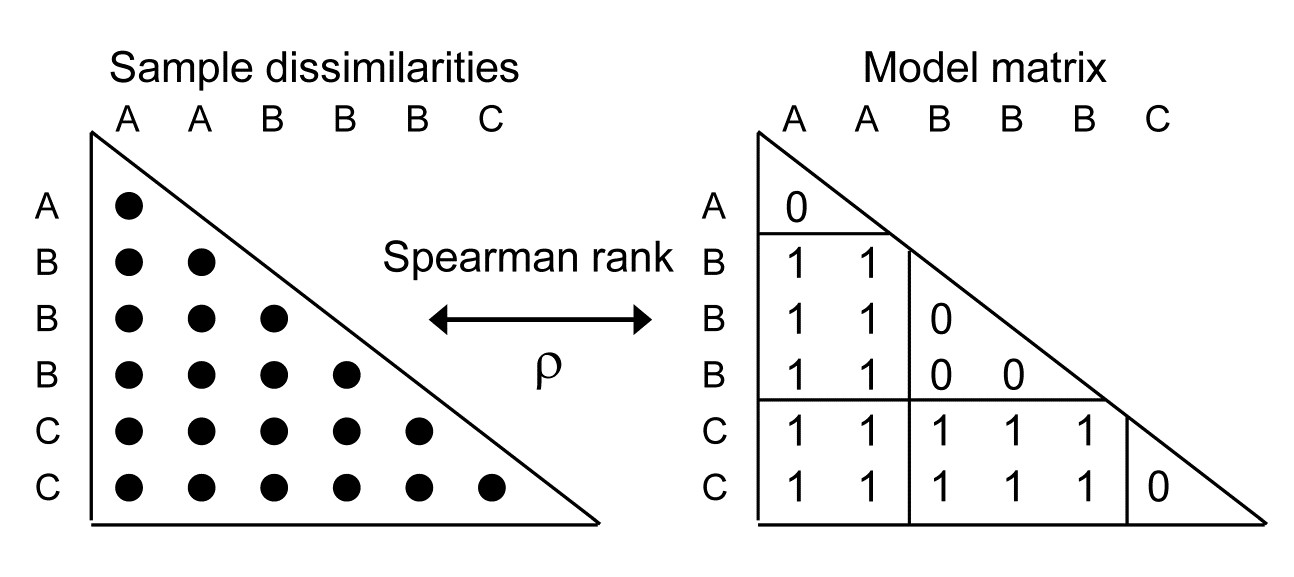
A RELATE $\rho$ statistic is not the same as an ANOSIM R statistic but the tests (which permute the labels over samples in the same way for the two tests) produce results which are identical because the two statistics are linked, in this simple case, by the relationship:
$$ R = \rho \sqrt{ \frac{ M^2 -1}{3w (M-w)}} \tag{6.6} $$
where w is the number of within-group ranks and M is the total number of ranks in the triangular matrix (thus for the simple example above, with groups A, B, C having replicates 2, 3, 2 respectively, w = 5, M = 21 and R = 1.35 $\rho$).
Importantly, there is a more fundamental relationship between the two statistics, which allows us to generalise the concept of an ANOSIM statistic to cater for ordered models. Then, the test is not of the null:
$$H_0: A = B = C = \ldots $$
against the general alternative
$$H_1: A, B, C, \ldots \text{ differ (in ways unspecified)}$$
but of the same null $H_0$ against an ordered alternative:
$$H_1: A < B < C < \ldots, $$
i.e. A & B and B & C are only one step apart but A & C are 2 steps (and A & D are 3 steps etc). This is an appropriate model for testing, say, for an inter-annual drift in an assemblage away from its initial state, or for serial change in community composition along an environmental gradient (e.g. with increasing water depth or away from a pollution source). The model matrix is now of the form:
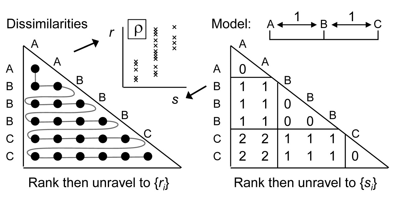
and the RELATE test is again the correlation $\rho$ of the dissimilarity ranks {$r_i$} against model ranks {$s_i$}. In contrast, the generalised ANOSIM statistic is defined totally generally as the slope of a linear regression of {$r_i$} on {$s_i$}, and denoted in the above ordered case by $R^O$ (the superscript upper case O denoting ‘ordered’). Testing of this statistic uses the appropriate permutation distribution; standard tests (or interval estimates) for the slope of the regression cannot be used because of the high degree of internal dependency among the {$r_i$} (dissimilarities are not mutually independent).
Several important points follow from this definition. Firstly, it takes only a few lines of algebra to show that, in the unordered case, this slope reduces to the usual ANOSIM R statistic. Secondly, the equations defining slopes and correlations dictate that $R^O$ is zero if and only if $\rho$ is zero, the null hypothesis condition. Thirdly, $R^O$ can never exceed 1 and it takes that value only under a generalisation of our standard ‘mantra’ for the (non-parametrically) most extreme multivariate separation that can be observed between groups, namely that ‘all dissimilarities between groups are larger than any within groups’, to which we must now add ‘and all dissimilarities between groups which are further apart in the model matrix are larger than any dissimilarities between groups which the model puts closer together’. This extreme case is illustrated by the following scatter plot for of {$r_i$} against {$s_i$} for the example above of three ordered groups A< B<C.

The absence of any overlap (or equality) of values on the y axis (for $r_i$) across the three possible tied ranks on the x axis ($s_i$ values) is what ensures that $R^O = 1$.
Fourthly, the model values {$s_i$} will always involve tied ranks in designs with replication (and also for simple trend models without replication), and the plot makes it clear that the correlation $\rho$ cannot in general attain its theoretical maximum of 1 (in all except pathological cases there has to be a scatter of y values at some x axis points). This makes $R^O$ potentially a more useful descriptor for these seriation with replication designs (as they are termed in Chapter 15, and Somerfield, Clarke & Olsgard (2002) ). Finally, one should note the asymmetry of the $R^O$ statistic relative to the symmetry of $\rho$. The generalised ANOSIM concept is restricted to regressing real data in the ranks {$r_i$} on modelled distances in the ranks {$s_i$}; it does not make sense to carry out the regression the other way round. The RELATE $\rho$ statistic, on the other hand, is appropriate for a wider sweep of problems where the interest is in comparing the sample patterns of any two triangular matrices¶; we have already met it used in this way, entirely symmetrically, in equation 6.3, and will do so repeatedly in later chapters.
¶ This contrast is also in part an issue of what to do about tied ranks, and identifies a context-dependent dichotomy noted early in the development of non-parametric methods ( Kendall (1970) ). Would we say that two judges were in perfect agreement only if they ranked 10 candidates in exactly the same order, or does placing the candidates into the same two groups of 5 ‘acceptable’ and 5 ‘not acceptable’ count as perfect agreement? In our case, $\rho$ (the former, which does not adjust for tied ranks) will be more appropriate for some problems, and generalised R (the latter, which does, in effect, build in an adjustment for ties in the {$s_i$}) more appropriate for other problems.