16.8 Example: Algal recolonisation, Calafuria
An example of this type (though not a classic BACI situation) is given by Clarke, Somerfield, Airoldi et al. (2006) , for a study by Airoldi (2000) . Sub-tidal patches of rocky reefs were cleared of algae at one station (Calafuria) on the Ligurian Sea coast of N Italy (data from two further stations is not shown here). Multiple marked (and interspersed) patches were cleared on 8 different months over the year 1995/6, and the time course of recolonisation examined at 6 times (c. bi-monthly) in the year following clearance, utilising non-destructive (photographic) estimates of % area cover by the algal species community. Data from three ‘patches’ (in fact these were themselves the average from three sub- patches) were tracked for each of the clearance start months (the ‘treatment’). One rationale for the design was to examine likely differences in recovery rates and patterns (after reef damage by shipping/boats) for the different times of year at which this may happen. It is clearly a repeated measures design, with the 6 bi-monthly samples of fixed patches being dependent.
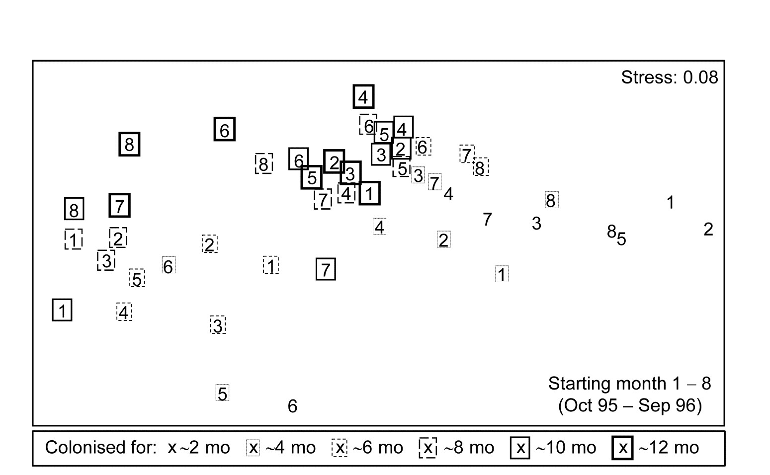
Fig. 16.15. Algal colonisation, Calafuria {a}. MDS of macroalgal species based on zero-adjusted Bray-Curtis from fourth-root transformed area cover, using photographs, for 48 samples, each an average over three replicate ‘patches’ (three sub-patches in each) for all $ 8 \times 6$ combinations of month of clearance (numbers 1-8 over the course of a year) and time over which colonisation has been taking place (six approximately bi-monthly sampling times, shown by a succession of larger/bolder boxes).
Fig. 16.15 is an nMDS of the 48 community samples, over 6 recovery periods (successively bolder squares) for the 8 different starting months of clearance (1-8), the three replicate patches for each ‘treatment’ (start date) having been averaged for this plot. Whilst a colonisation pattern through time is evident (mid-right to low left then upwards) there is no prospect of seeing whether that pattern is the same across the start times since assemblage differences are naturally large over the colonisation period. The trajectories of the 6 times for each of the patches, viewed separately by MDS ordination in their groups of three patches per treatment (Fig. 16.16), do however show strong differences in these time profiles. Though they are spatially interspersed, there is a marked consistency of replicate patches within treatments and characteristically different colonisation profiles across them.
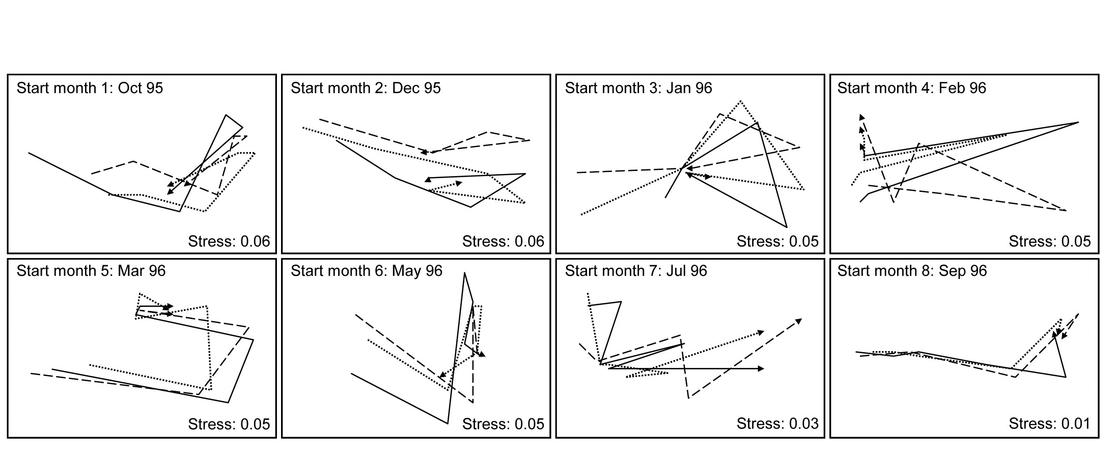
Fig. 16.16. Algal recolonisation, Calafuria {a}. Separate nMDS plots for each of the 8 clearance months (‘treatments’), showing time trajectories over the following 6 approximately bi-monthly observations of the colonising macroalgal communities, for three replicate patches in each treatment (different line shading). Note the similarity of trajectories within, and dissimilarity between, treatments.
With outer factor the patch designators and inner factor the 6 bi-monthly times, the 2STAGE routine extracts the $6 \times 6$ similarity matrix representing each profile, from diagonals of the $144 \times 144$ Bray-Curtis matrix for the full set of samples, and then relates the 24 such sub-matrices with rank matrix correlations $\rho$, each sub-matrix then becoming a single point in the second-stage nMDS of Fig. 16.17. Unlike the earlier coral reef example, there are now replicates which will allow a formal hypothesis test, and ANOSIM on the differences among starting times assessed against the variability over replicate patches (in their time profiles, not in their communities!) gives a decisive global R of 0.96.¶ By averaging over the replicate level, Clarke, Somerfield, Airoldi et al. (2006) go on to demonstrate that the experiment is repeatable, since the second-stage pattern of the 8 starting months at the Calafuria station is strongly related to the pattern for the same sampling design at another station, Boccale. This utilises a RELATE test on the two second-stage matrices, a procedure which comes dangerously close to being a third-stage analysis, by which point the original data has become merely a distant memory!
The serious point here, of course, is that plots such as Fig. 16.17 are never the end point of a multivariate analysis. They may help to tease out, and sometimes formally test, interesting and relevant assemblage patterns, but having established that there are valid interpretations to be made, a return to the data matrix is always desirable, and the types of species analyses covered in Chapter 7 (much enhanced in PRIMER v7) will then usually play an important part in the final interpretation.
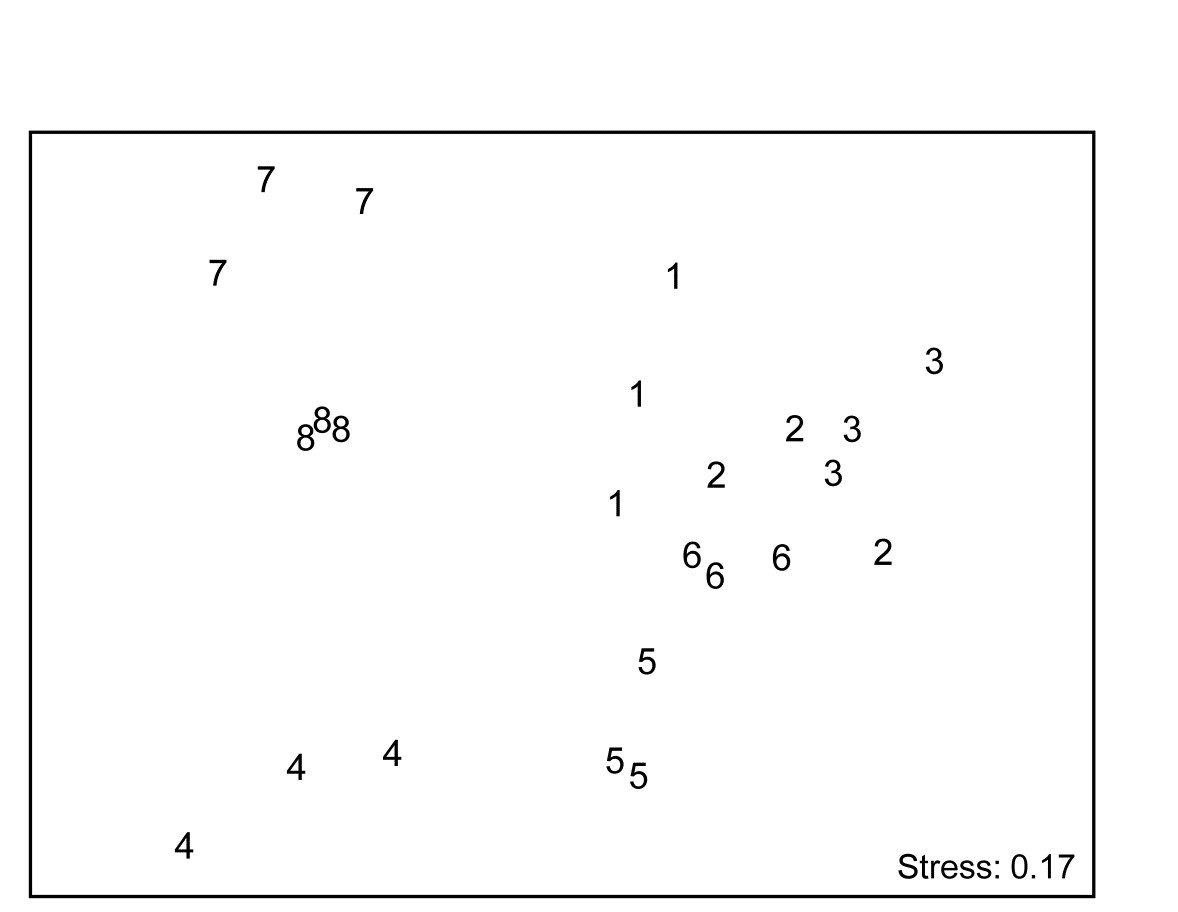
Fig. 16.17. Algal recolonisation, Calafuria {a}. Second-stage nMDS of similarities in the time course of recolonisation of macroalgae, as seen in the first-stage MDS plots of Fig. 16.16, i.e. at 3 ‘patches’ under 8 different months (1-8) of clearance of algae from the subtidal rocky reefs (the ‘treatments’). The very consistent time course within, and marked differences between, treatments is seen in the tight dispersion of the replicates, giving a large and highly significant ANOSIM statistic, R = 0.96.
¶ In fact, had the nested design of smaller patches within each of these replicate ‘patches’ been exploited, the second-stage tests at this point would have been 2-way nested ANOSIM.