6.9 Example: Exe nematodes (no replication and missing data)

A final example demonstrates a positive outcome to such a test, in a common case of a 2-way layout of sites and times with the additional feature that samples are missing altogether from a small number of cells. Fig. 6.11 shows again the MDS, from Chapter 5, of nematode communities at 19 sites in the Exe estuary.

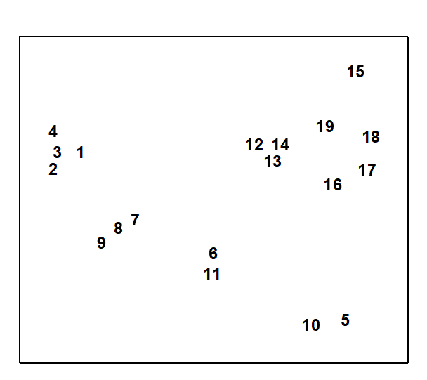
Fig. 6.11. Exe estuary nematodes {X}. MDS, for 19 inter-tidal sites, of species abundances averaged over 6 bi-monthly sampling occasions; see also Fig.5.1 (stress = 0.05).
 

In fact, this is based on an average of data over six successive bi-monthly sampling occasions. For the individual times, the samples remain strongly clustered into the 4 or 5 main groups apparent from Fig. 6.11. Less clear, however, is whether any structure exists within the largest group (sites 12 to 19) or whether their scatter in Fig. 6.11 is just sampling variation.

Rejection of the null hypothesis of ‘no site differences’ would be suggested by a common site pattern in the separate MDS plots for the 6 times (Fig. 6.12). At some of the times, however, one of the site samples is missing (site 19 at times 1 and 2, site 15 at time 4 and site 18 at time 6). Instead of removing these sites from all plots, in order to achieve matching sets of similarities, one can remove for each pair of times only those sites missing for either of that pair, and compute the Spearman correlation $\rho$ between the remaining rank similarities. The $\rho$ values for all pairs of times are then averaged to give $\rho_{av}$, i.e. the left-hand route is taken in the lower half of Fig. 6.9. This is usually referred to as pairwise removal of missing data, in contrast to the listwise removal that would be needed for the right-hand route. Though increasing the computation time, pairwise removal clearly utilises more of the available information.

Fig. 6.12 shows evidence of a consistent site pattern, for example in the proximity of sites 12 to 14 and the tendency of site 15 to be placed on its own; the fact that site 15 is missing on one occasion does not undermine this perceived structure. Pairwise computation gives $\rho _ {av} = 0.36$ and its significance can be determined by a permutation test, as before. The (non-missing) site labels are permuted amongst the available samples, separately for each time, and these designations fixed whilst all the paired r values are computed (using pairwise removal) and averaged. Here the, largest such $\rho _ {av}$ value in 999 simulations was 0.30, so the null hypothesis is rejected at the p<0.1% level.

In the same way, one can also carry out a test of the hypothesis that there are no differences across time for sites 12 to 19. The component plots, of the 4 to 6 times for each site, display no obvious features and rav = 0.08 (p<18%). The failure to reject this null hypothesis justifies the use of averaged data across the 6 times, in the earlier analyses, and could even be thought to justify use of times as ‘replicates’ for sites in a 1-way ANOSIM test for sites.

Tests of this form, searching for agreement between two or more similarity matrices, occur also in Chapter 11 (in the context of matching species to environmental data) and Chapter 15 (where they link biotic patterns to some model structure). The discussion there includes use of measures other than a simple Spearman coefficient, for example a weighted Spearman coefficient $\rho _ w$ (suggested for reasons explained in Chapter 11), and these adjustments could certainly be implemented here also if desired, using the left-hand route in the lower half of Fig.6.9. In the present context, this type of ‘matching’ test is clearly an inferior one to that possible where genuine replication exists within the 2-way layout. It cannot cope with follow-up tests for differences between specific pairs of treatments, and it can have little sensitivity if the numbers of treatments and blocks are both small. A test for two treatments is impossible note, since the treatment pattern in all blocks would be identical.

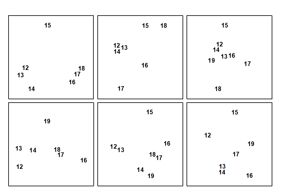
Fig. 6.12. Exe estuary nematodes {X}. MDS for sites 12 to 19 only, performed separately for the 6 sampling times (read across rows for time order); in spite of the occasional missing sample some commonality of site pattern is apparent (stress ranges from 0.01 to 0.08).