6.3 Example: Frierfjord macrofauna
The rank similarities underlying Fig. 6.3 are shown in Table 6.2 (note that these are the similarities involving only sites B, C and D, extracted from the matrix for all sites and re-ranked). Averaging across the 3 diagonal sub-matrices (within groups B, C and D) gives $\overline{r}_W = 22.7$, and across the remaining (off-diagonal) entries gives $\overline{r}_B = 37.5$. Also $n = 12$ and $M = 66$, so that $R = 0.45$. In contrast, the spread of R values possible from random re-labelling of the 12 samples can be seen in the histogram of Fig. 6.4: the largest of $T = 999$ simulations is less than 0.45 ($t = 0$). An observed value of $R = 0.45$ is seen to be a most unlikely event, with a probability of less than 1 in a 1000 if H$_o$ is true, and we can therefore reject H$_o$ at a significance level of p<0.1% (at least, because $R = 0.45$ may still have been the most extreme outcome observed had we chosen an even larger number of permutations. If it is the most extreme of all 5775 – it will be one of them – then p = 100(1/5775) = 0.02%).
Table 6.2. Frierfjord macrofauna {F}. Rank similarity matrix for the 4 replicates from each of B, C and D, i.e. C3 and C4 are the most, and B1 and C1 the least, similar samples.
| B1 | B2 | B3 | B4 | C1 | C2 | C3 | C4 | D1 | D2 | D3 | D4 | |
|---|---|---|---|---|---|---|---|---|---|---|---|---|
| B1 | – | |||||||||||
| B2 | 33 | – | ||||||||||
| B3 | 8 | 7 | – | |||||||||
| B4 | 22 | 11 | 19 | – | ||||||||
| C1 | 66 | 30 | 58 | 65 | – | |||||||
| C2 | 44 | 3 | 15 | 28 | 29 | – | ||||||
| C3 | 23 | 16 | 5 | 38 | 57 | 6 | – | |||||
| C4 | 9 | 34 | 4 | 32 | 61 | 10 | 1 | – | ||||
| D1 | 48 | 17 | 42 | 56 | 37 | 55 | 51 | 62 | – | |||
| D2 | 14 | 20 | 24 | 39 | 52 | 46 | 35 | 36 | 21 | – | ||
| D3 | 59 | 49 | 50 | 64 | 54 | 53 | 63 | 60 | 43 | 41 | – | |
| D4 | 40 | 12 | 18 | 45 | 47 | 27 | 26 | 31 | 25 | 2 | 13 | – |
Pairwise tests
The above is a global test, indicating that there are site differences somewhere that may be worth examining further. Specific pairs of sites can then be compared: for example, the similarities involving only sites B and C are extracted, re-ranked and the test procedure repeated, giving an R value of 0.23. This time there are only 35 distinct relabellings so, under the null hypothesis H$ _ o$ that sites B and C do not differ, the full permutation distribution of possible values of R can be computed; 12% of these values are equal to or larger than 0.23 so H$ _ o$ cannot be rejected. By contrast, R = 0.54 for the comparison of B against D, which is the most extreme value possible under the 35 permutations. B and D are therefore inferred to differ significantly at the p< 3% level. For C against D, R = 0.57 similarly leads to rejection of the null hypothesis (p<3%).
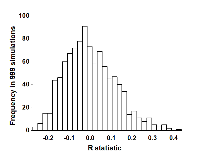
Fig. 6.4. Frierfjord macrofauna {F}. Permutation distribution of the test statistic R (equation 6.1) under the null hypothesis of ‘no site differences’; this contrasts with an observed value for R of 0.45.
There is a danger in such repeated significance tests which should be noted (although rather little can be done to ameliorate it here). To reject the null hypothesis at a significance level of 3% implies that a 3% risk is being run of drawing an incorrect conclusion (a Type I error in statistical terminology). If many such tests are performed this risk will cumulate. For example, all pairwise comparisons between 10 sites, each with 4 replicates (allowing 3% level tests at best), would involve 45 tests, and the overall risk of drawing at least one false conclusion is high. For the analogous pairwise comparisons following the global F test in a univariate ANOVA, there exist multiple comparison tests which attempt to adjust for this repetition of risk. One straightforward possibility, which could be carried over to the present multivariate test, is a Bonferroni correction. In its simplest form, this demands that, if there are n pairwise comparisons in total, each test uses a significance level of 0.05/n. The so-called experiment-wise Type I error, the overall probability of rejecting the null hypothesis at least once in the series of pairwise tests, when there are no genuine differences, is then kept to 0.05.
However, the difficulty with such a Bonferroni correction is clear from the above example: with only 4 replicates in each group, and thus only 35 possible permutations, a significance level of 0.05/3 (=1.7%) can never be achieved! It may be possible to plan for a modest improvement in the number of replicates: 5 replicates from each site would allow a 1% level test for a pairwise comparison, equation (6.2) showing that there are then 126 permutations, and two groups of 6 replicates would give close to a 0.2% level test. However, this may not be realistic in some practical contexts, or it may be inefficient to concentrate effort on too many replicates at one site, rather than (say) increasing the spatial coverage of sites. Also, for a fixed number of replicates, a too demandingly low Type I error (significance level) will be at the expense of a greater risk of Type II error, the probability of not detecting a difference when one genuinely exists.
Strategy for interpretation
The solution, as with all significance tests, is to treat them in a more pragmatic way, exercising due caution in interpretation certainly, but not allowing the formality of a test procedure for pairwise comparisons to interfere with the natural explanation of the group differences. Herein lies the real strength of defining a test statistic, such as R, which has an absolute interpretation of its value†. This is in contrast to a standard Z-type statistic, which typically divides an appropriate measure (taking the value zero under the null hypothesis) by its standard deviation, so that interpretation is limited purely to statistical significance of the departure from zero.
The recommended course of action, for a case such as the above Frierfjord data, is therefore always to carry out, and take totally seriously, the global ANOSIM test for overall differences between groups. Usually the total number of replicates, and thus possible permutations, is relatively large, and the test will be reliable and informative. If it is not significant, then generally no further interpretation is permissible. If it is significant, it is legitimate to ask where the main between-group differences have arisen. The best tool for this is an examination of the R value for each pairwise comparison: large values (close to unity) are indicative of complete separation of the groups, small values (close to zero) imply little or no segregation. If the MDS is of sufficiently low stress to give a reliable picture, then the relative group separations will also be evident from this.¶ The R value itself is not unduly affected by the number of replicates in the two groups being compared; this is in stark contrast to its statistical significance, which is dominated by the group sizes (for large numbers of replicates, R values near zero could still be deemed ‘significant’, and conversely, few replicates could lead to R values close to unity being classed as ‘non-significant’).
The analogue of this approach in the univariate case (say in the comparison of species richness between sites) would be firstly to compute the global F test for the ANOVA. If this establishes that there are significant overall differences between sites, the size of the effects would be ascertained by examining the differences in mean values between each pair of sites, or equivalently, by simply looking at a plot of how the mean richness varies across sites (usually without the replicates also shown). It is then immediately apparent where the main differences lie, and the interpretation is a natural one, emphasising the important biological features (e.g. absolute loss in richness is 5, 10, 20 species, or relative loss is 5%, 10%, 20% of the species pool, etc), rather than putting the emphasis solely on significance levels in pairwise comparisons of means that run the risk of missing the main message altogether.
So, returning to the multivariate data of the above Frierfjord example, interpretation of the ANOSIM tests is seen to be straightforward: a significant level (p<0.1%) and a mid-range value of R (= 0.45) for the global test of sites B, C and D establishes that there are statistically significant differences between these sites. Similarly mid-range values of R (slightly higher, at 0.54 and 0.57) for the B v D and C v D comparisons, contrasted with a much lower value (of 0.27) for B v C, imply that the explanation for the global test result is that D differs from both B and C, but the latter sites are not distinguishable.
The above discussion has raised the issue of Type II error for an ANOSIM permutation test, and the complementary concept, that of the power of the test, namely the probability of detecting a difference between groups when one genuinely exists. Ideas of power are not easily examined for non-parametric procedures of this type, which make no distributional assumptions and for which it is difficult to specify a precise non-null hypothesis. All that can be obviously said in general is that power will improve with increasing replication, and some low levels of replication should be avoided altogether. For example, if comparing only two groups with a 1-way ANOSIM test, based on only 3 replicates for each group, then there are only 10 distinct permutations and a significance level better than 10% could never be attained. A test demanding a significance level of 5% would then have no power to detect a difference between the groups, however large that difference is!
Generality of application
It is evident that few, if any, assumptions are made about the data in constructing the 1-way ANOSIM test, and it is therefore very generally applicable. It is not restricted to Bray-Curtis similarities or even to similarities computed from species abundance data: it could provide a non-parametric alternative to Wilks’ $\Lambda$ test for data which are more nearly multivariate-normally distributed, e.g. for testing whether groups (sites or times) can be distinguished on the basis of their environmental data (see Chapter 11). The latter would involve computing a Euclidean distance matrix between samples (after suitable transformation and normalising of the environmental variables) and entry of this distance matrix to the ANOSIM procedure. Clearly, if multivariate normality assumptions are genuinely justified then the ANOSIM test must lack sensitivity in comparison with standard MANOVA, but this would seem to be more than compensated for by its greater generality.
Note also that there is no restriction to a balanced number of replicates. Some groups could even have only one replicate provided enough replication exists in other groups to generate sufficient permutations for the global test (though there will be a sense in which the power of the test is compromised by a markedly unbalanced design, here as elsewhere). More usefully, note that no assumptions have been made about the variability of within-group replication needing to be similar for all groups. This is seen in the following example, for which the groups in the 1-way layout are not sites but samples from different years at a single site.
† A standard correlation coefficient, r, would be another example, like ANOSIM R, of a statistic which is both a test statistic (for the null hypothesis of absence of correlation, r = 0) and which has an interpretation as an effect size (large r is strong correlation).
¶ But the comparison of ANOSIM R values is the more generally valid approach, e.g. when the two descriptions do not appear to be showing quite the same thing. Calculation of R is in no way dependent on whether the 2-dimensional approximation implicit in an MDS is satisfactory or not, since R is computed from the underlying, full-dimensional similarity matrix.