5.9 Example: Okura estuary macrofauna
Anderson, Ford, Feary et al. (2004) describe macrofauna samples from the Okura estuary {O}, on the northern fringes of urban Auckland, NZ, taken inter-tidally at 2 times in each of 3 seasons under 3 sedimentary regimes (High, Medium and Low sedimentation levels), each regime represented by 5 sites, with 6 cores taken per site at each time. Taking averages¶ of log(x+1) transformed abundances over the sets of 30 site $\times$ replicate samples gives a very robust estimate of the community structure at each of the 18 time $\times$ sedimentation levels. However, calculating Bray-Curtis similarities then leads to the collapsed nMDS plot of Fig. 5.13a, since all dissimilarities between the highest and lower sedimentation levels (H compared with L and M) are greater than 40 and those within either of these two groups are all less than 30. The two sub-plots can be extracted, as shown in insets to Fig. 5.13a (simply achieved in PRIMER by drawing a box round each collapsed point and taking the ‘MDS subset’ routine), but it is more instructive to retain these averages on the same ordination. Just a small amount of metric stress here (5%, though the solution is robust to a wide range of values for the mixing proportion) is enough to calibrate the relative dissimilarities between the two sedimentation regimes (H and L/M) to those within them, Fig. 5.13b. The Shepard plots (c and d) show the contrast between a solution which is degenerate and a valid nMDS ordination: the disjunction in dissimilarities which forced the original collapse is very clear in both plots. As emphasised by Anderson, Gorley & Clarke (2008) ) the advantage of the single ordination is seen in the way the seasonal ordering (1=winter/spring, 2=spring/summer, 3=late summer) is matched, across the (large) sedimentation divide.
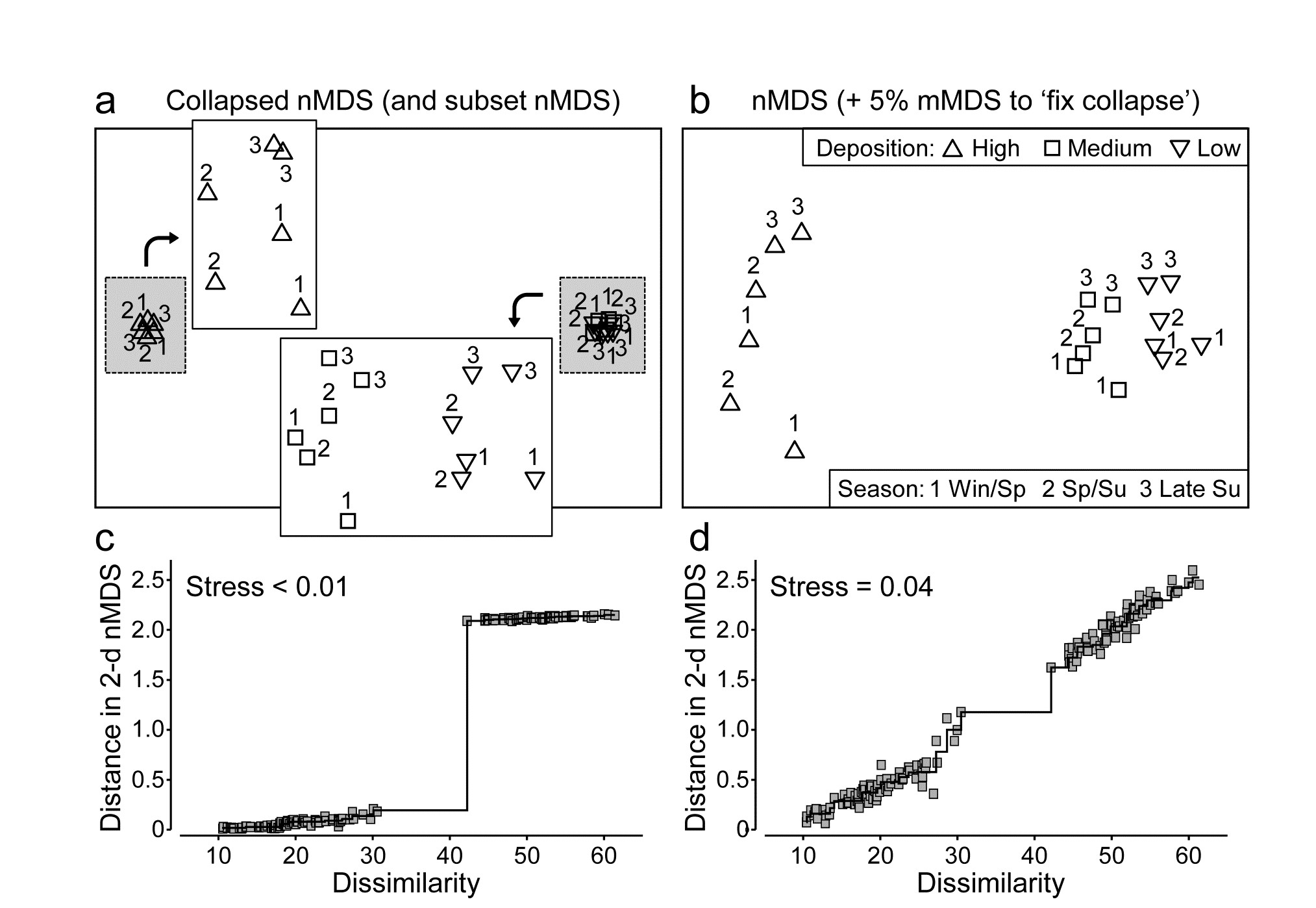
Fig. 5.13. Okura macrofauna {O}. a&c) Collapsed nMDS and associated Shepard plot from Bray-Curtis similarities on averages over 30 samples of log transformed abundances of 73 taxa, for 2 times in each season (1-3: Winter-Spring, Spring-Summer and Late Summer) and 3 levels of sedimentation (High, Medium, Low). Stress$\rightarrow 0$ for collapsed nMDS; subset nMDS plots for H and L/M separately (insets in a) have stress = 0.04, 0.07.
b&d) nMDS for Fix Collapse option (stress defined as mix 0.95$\times$nMDS + 0.05$\times$mMDS), and the Shepard plot for that nMDS, with stress 0.04.
Combining data sets
Another context in which we might want to combine MDS solutions into a single ordination, which optimises their combined stress function, arises when there is no clear way of merging two data sets with exactly the same sample labels (same times, sites, treatments etc) but of very different type. For example, in rocky shores, counts might be made of motile species but area cover of sessile or colonial organisms, and it may be hard to reconcile those two types of measurement in a single array. The classic solution to mixed measurement scales is to normalise variables but this gives each species an equal contribution in defining resemblance, irrespective of their total counts or area cover, and this may be very undesirable (it can add a great deal of ‘noise’ from rare species); it is much better to keep the natural internal weightings for each species. Perhaps the best solution is to convert both matrices onto a common scale (such as biomass or ‘equivalent area cover’) and merge them into a single array, but an alternative worth considering is to run a combined nMDS (an option under PRIMER7) which fits separate Shepard plots for each matrix to common ordination co-ordinates, minimising the average of the two stress values. The result is an equal mix of the two sets of information on sample relationships.
Note that it is inevitable that the resulting stress value will be higher than for either of the separate nMDS ordinations, since it must represent a compromise of two potentially conflicting sets of relationships; it can only come close to the stress in the separate plots if they have effectively identical patterns. (The same is not true of merging the two matrices into a single array, of course, because there the compromise is effected in the calculation of the resemblances).
An example of where a merged matrix is usually not possible but a combined nMDS is a viable solution is where the matrices to combine require very different dissimilarity measures, such as for assemblage counts (e.g. Bray-Curtis) and environmental variables which may be driving those counts (e.g. Euclidean distance). Arguably, there are few convincing examples of why a compromise MDS is a desirable output here (rather than adopting the approach in Chapter 11 that we let the two components ‘speak for themselves’ and then seek variables, or sets of variables, which ‘explain’ the biotic patterns) but an example is given below of the result of a combined MDS, were it to be needed.
¶ This example is taken from the PERMANOVA+ manual, Anderson, Gorley & Clarke (2008) . There, the ‘averages’ are the (theoretically more correct) centroids in the high-dimensional ‘Bray-Curtis space’ from the full 540 samples, i.e. averaging is performed after similarity calculation not before. Whilst data averages are not the same as centroids from dissimilarity space (e.g. an averaged assemblage may not be ‘central’ to individual samples, since it will usually have higher species richness), it is commonly found that the relationship amongst averages can be very similar to the relationship amongst centroids, as is seen here when comparing Fig. 5.13a with the PCO of Fig. 3.13 in Anderson, Gorley & Clarke (2008) .