5.2 Non-metric multidimensional scaling (MDS)
The method of non-metric MDS was introduced by Shepard (1962) and Kruskal (1964) , for application to problems in psychology; a useful introductory text is Kruskal & Wish (1978) , though the applications given are not ecological. Generally, we use the term MDS to refer to Kruskal’s non-metric procedure (though if there is any risk of confusion, nMDS is used). Metric MDS (always mMDS) is generally less useful but will be discussed in specific contexts later in the chapter.
The starting point is the resemblance matrix among samples (Chapter 2). This can be whatever similarity matrix is biologically relevant to the questions being asked of the data. Through choice of coefficient and possible transformation or standardisation, one can choose whether to ignore joint absences, emphasise similarity in common or rare species, compare only % composition or allow sample totals to play a part, etc. In fact, the flexibility of (n)MDS goes beyond this. It recognises the essential arbitrariness of absolute similarity values: Chapter 2 shows that the range of values taken can alter dramatically with transformation (often, the more severe the transformation, the higher and more compressed the similarity values become). There is no clear interpretation of a statement like ‘the similarity of samples 1 and 2 is 25 less than, or half that of, samples 1 and 3’. A transparent interpretation, however, is in terms of the rank values of similarity to each other, e.g. simply that ‘sample 1 is more similar to sample 2 than it is to sample 3’. This is an intuitively appealing and very generally applicable base from which to build a graphical representation of the sample patterns and, in effect, the ranks of the similarities are the only information used by a non-metric MDS ordination.
The purpose of MDS can thus be simply stated: it constructs a ‘map’ or configuration of the samples, in a specified number of dimensions, which attempts to satisfy all the conditions imposed by the rank (dis)similarity matrix, e.g. if sample 1 has higher similarity to sample 2 than it does to sample 3 then sample 1 will be placed closer on the map to sample 2 than it is to sample 3.
Example: Loch Linnhe macrofauna
This is illustrated in Table 5.1 for the subset of the Loch Linnhe macrofauna data used to show hierarchical clustering (Table 3.2). Similarities between $\sqrt{} \sqrt{}$-transformed counts of the four year samples are given by Bray-Curtis similarity coefficients, and Table 5.1 then shows the corresponding rank similarities. (The highest similarity has the lowest rank, 1, and the lowest similarity the highest rank, n(n-1)/2.) The MDS configuration is constructed to preserve the similarity ranking as Euclidean distances in the 2-dimensional plot: samples 2 and 4 are closest, 2 and 3 next closest, then 1 and 4, 3 and 4, 1 and 2, and finally, 1 and 3 are furthest apart. The resulting figure is a more informative summary than the corresponding dendrogram in Chapter 3, showing, as it does, a gradation of change from clean (1) to progressively more impacted years (2 and 3) then a reversal of the trend, though not complete recovery to the initial position (4).
Though the mechanism for constructing such MDS plots has not yet been described, two general features of MDS can already be noted:
-
MDS plots can be arbitrarily scaled, located, rotated or inverted. Clearly, rank order information about which samples are most or least similar can say nothing about which direction in the MDS plot is up or down, or the absolute distance apart of two samples: what is interpretable is relative distances apart, in whatever direction.
-
It is not difficult in the above example to see that four points could be placed in two dimensions in such a way as to satisfy the similarity ranking perfectly.‡ For more realistic data sets, though, this will not usually be possible and there will be some distortion (stress) between the similarity ranks and the corresponding distance ranks in the ordination. This motivates the principle of the MDS algorithm: to choose a configuration of points which minimises this degree of stress, appropriately measured.
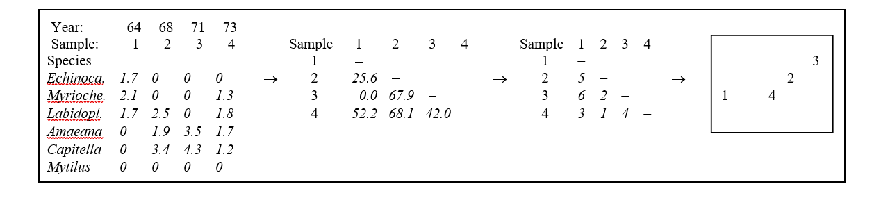
Table 5.1. Loch Linnhe macrofauna {L} subset. Abundance array after $\sqrt{} \sqrt{}$-transform, the Bray-Curtis similarities (as in Table 3.2), the rank similarity matrix and the resulting 2-dimensional MDS ordination.
Example: Exe estuary nematodes
The construction of an MDS plot is illustrated with data collected by Warwick (1971) and subsequently analysed in this way by Field, Clarke & Warwick (1982) . A total of 19 sites from different locations and tide-levels in the Exe estuary, UK, were sampled bi-monthly at low spring tides over the course of a year, between October 1966 and September 1967.
Three replicate sediment cores were taken for meiofaunal analysis on each occasion, and nematodes identified and counted. This analysis here considers only the mean nematode abundances across replicates and season (seasonal variation was minimal) and the matrix consists of 140 species found at the 19 sites.
This is not an example of a pollution study: the Exe estuary is a relatively pristine environment. The aim here is to display the biological relationships among the 19 stations and later to link these to the environmental variables (granulometry, interstitial salinity etc.) measured at these sites, to reveal potential determinants of nematode community structure. Fig. 5.1 shows the 2-dimensional MDS ordination of the 19 samples, based on $\sqrt{} \sqrt{}$-transformed abundances and a Bray-Curtis similarity matrix. Distinct clusters of sites emerge (in agreement with those from a matching cluster analysis), bearing no clear-cut relationship to geographical position or tidal level of the samples. Instead, they appear to relate to sediment characteristics and these links are discussed in Chapter 11. For now the question is: what are stages in the construction of Fig. 5.1?
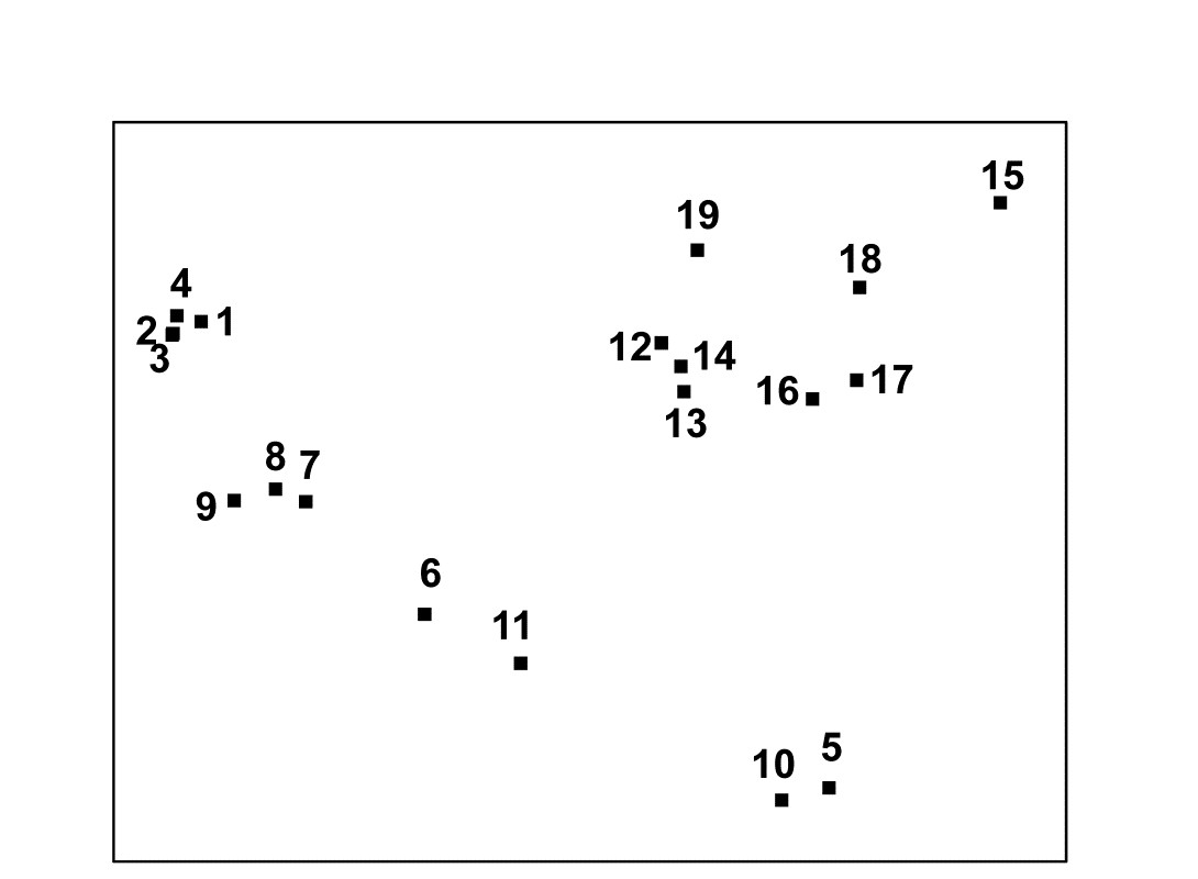
Fig. 5.1. Exe estuary nematodes {X}. MDS ordination of the 19 sites based on √√-transformed abundances and Bray-Curtis similarities (stress = 0.05).
MDS algorithm
The non-metric MDS algorithm, as first employed in Kruskal’s original MDSCAL program for example, is an iterative procedure, constructing the MDS plot by successively refining the positions of the points until they satisfy, as closely as possible, the dissimilarity relations between samples.§ It has the following steps.
-
Specify the number of dimensions (m) required in the final ordination. If, as will usually be desirable, one wishes to compare configurations in different dimensions then they have to be constructed one at a time. For the moment think of m as 2.
-
Construct a starting configuration of the n samples. This could be the result of an ordination by another method, for example PCA or PCO, but there are advantages in using just a random set of n points in m (=2) dimensions.
-
Regress the interpoint distances from this plot on the corresponding dissimilarities. Let {$d _ {jk}$} denote the distance between the jth and kth sample points on the current ordination plot, and {$\delta _ {jk}$} the corresponding dissimilarity in the original dissimilarity matrix (e.g. of Bray-Curtis coefficients, or whatever resemblance measure is relevant to the context). A scatter plot is then drawn of distance against dissimilarity for all n(n–1)/2 such pairs of values. This is termed a Shepard diagram and Fig. 5.2 shows the type of graph that results. (In fact, Fig. 5.2 is at a late stage of the iteration, corresponding to the final 2-dimensional configuration of Fig. 5.1; at earlier stages the graph will appear similar though with a greater degree of scatter). The decision that characterises different ordination procedures must now be made: how does one define the underlying relation between distance in the plot and the original dissimilarity?
There are two main approaches.
a) Fit a standard linear regression of $d$ on $\delta$, so that final distance is constrained to be proportional to original dissimilarity. This is metric MDS (mMDS). (More flexible would be to fit some form of curvilinear regression model, termed parametric MDS, though this is rarely seen.)
b) Perform a non-parametric regression of $d$ on $\delta$ giving rise to non-metric MDS. Fig. 5.2 illustrates the non-parametric (monotonic) regression line. This is a ‘best-fitting’ step function which moulds itself to the shape of the scatter plot, and at each new point on the x axis is always constrained to either remain constant or step up. The relative success of non-metric MDS, in preserving the sample relationships in the distances of the ordination plot, comes from the flexibility in shape of this non-parametric regression line. A perfect MDS was defined before as one in which the rank order of dissimilarities was fully preserved in the rank order of distances. Individual points on the Shepard plot must then all be monotonic increasing: the larger a dissimilarity, the larger (or equal) the corresponding distance, and the non-parametric regression line is a perfect fit. The extent to which the scatter points deviate from the line measures the failure to match the rank order dissimilarities, motivating the following.
-
Measure goodness-of-fit of the regression by a stress coefficient (Kruskal’s stress formula 1):
$$ Stress = \sqrt{ \sum_j \sum_k ( d_ {jk} - \hat{d}_ {jk} ) ^ 2 / \sum_j \sum_k d _ {jk}^2 } \tag{5.1} $$
where $\hat{d} _ {jk}$ is the distance predicted from the fitted regression line corresponding to dissimilarity $\delta _ {jk}$. If $d _ {jk} = \hat{d} _ {jk}$ for all the n(n–1)/2 distances in this summation, the stress is zero. Large scatter clearly leads to large stress and this can be thought of as measuring the difficulty involved in compressing the sample relationships into two (or a small number) of dimensions. Note that the denominator is simply a scaling term: distances in the final plot have only relative not absolute meaning and the squared distance term in the denominator makes sure that stress is a dimensionless quality.
-
Perturb the current configuration in a direction of decreasing stress. This is perhaps the most difficult part of the algorithm to visualise and will not be detailed; it is based on established techniques of numerical optimisation, in particular the method of steepest descent. The key idea is that the regression relation is used to calculate the way stress changes for small changes in the position of individual points on the ordination, and points are then moved to new positions in directions which look like they will decrease the stress most rapidly.
-
Repeat steps 3 to 5 until convergence is achieved. The iteration now cycles around the two stages of a new regression of distance on dissimilarity for the new ordination positions, then further perturbation of the positions in directions of decreasing stress. The cycle stops when adjustment of points leads to no further improvement in stress¶ (or when, say, 100 such regression/steepest descent/regression/… cycles have been performed without convergence).
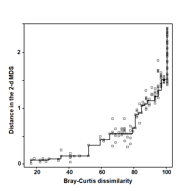
Fig. 5.2. Exe estuary nematodes {X}. Shepard diagram of the distances (d) in the MDS plot (Fig. 5.1) against the dissimilarities ($\delta$) in the Bray-Curtis matrix. The line is the fitted non-parametric regression; stress (=0.05) is a measure of scatter about the line in the vertical direction.
Features of the algorithm
Local minima. Like all iterative processes, especially ones this complex, things can go wrong! By a series of minor adjustments to the parameters at its disposal (the co-ordinate positions in the configuration), the method gradually finds its way down to a minimum of the stress function. This is most easily envisaged in three dimensions, with just a two-dimensional parameter space (the x, y plane) and the vertical axis (z) denoting the stress at each (x, y) point. In reality the stress surface is a function of more parameters than this of course, but we have seen before how useful it can be to visualise high-dimensional algebra in terms of three-dimensional geometry. A relevant analogy is to imagine a rambler walking across a range of hills in a thick fog, attempting to find the lowest point within an encircling range of high peaks. A good strategy is always to walk in the direction in which the ground slopes away most steeply (the method of steepest descent, in fact) but there is no guarantee that this strategy will necessarily find the lowest point overall, i.e. the global minimum of the stress function. The rambler may reach a low point from which the ground rises in all directions (and thus the steepest descent algorithm converges) but there may be an even lower point on the other side of an adjacent hill. He is then trapped in a local minimum of the stress function. Whether he finds the global or a local minimum depends very much on where he starts the walk, i.e. the starting configuration of points in the ordination plot.
Such local minima do occur routinely in all MDS analyses, usually corresponding to configurations of sample points which are only slightly different to each other. Sometimes this may be because there are one or two points which bear little relation to any of the other samples and there is a choice as to where they may best be placed, or perhaps they have a more complex relationship with other samples and may be difficult to fit into (say) a 2-dimensional picture.
There is no guaranteed method of ensuring that a global minimum of the stress function has been reached; the practical solution is therefore to repeat the MDS analysis several times starting with different random positions of samples in the initial configuration (step 2 above). If the same (lowest stress) solution re-appears from a number of different starts then there is a strong assurance, though never a guarantee, that this is indeed the best solution. Note that the easiest way to determine whether the same solution has been reached as in a previous attempt is simply to check for equality of the stress values; remember that the configurations themselves could be arbitrarily rotated or reflected with respect to each other.† In genuine applications, converged stress values are rarely precisely the same if configurations differ. (Outputting stress values to 3 d.p. can help with this, though solutions which are the same to 2 d.p. will be telling you the same story, in practice).
Degenerate solutions can also occur, in which groups of samples collapse to the same point (even though they are not 100% similar), or to the vertices of a triangle, or strung out round a circle. In these cases the stress may go to zero. (This is akin to our rambler starting his walk outside the encircling hills, so that he sets off in totally the wrong direction and ends up at the sea!). Artefactual solutions of this sort are relatively rare and easily seen in the MDS plot and the Shepard diagram (the latter may have just a single step at one end): repetition from different random starts will find many solutions which are sensible. (In fact, a more likely cause of a plot in which points tend to be placed around the circumference of a circle is that the input matrix is of similarities when the program has been told to expect dissimilarities, or vice-versa; in such cases the stress will be very high.)
A much more common form of degenerate solution is repeatable and is a genuine result of a disjunction in the data. For example, if the data split into two well-separated groups for which dissimilarities between the groups are much larger than any within either group, then there may be no yardstick within our rank-based approach for determining how far apart the groups should be placed in the MDS plot. Any solution which places the groups ‘far enough’ apart to satisfy the conditions may be equally good, and the algorithm can then iterate to a point where the two groups are infinitely far apart, i.e. the group members collapse on top of each other, even though they are not 100% similar (a commonly met special case is when one of the two groups consists of a single outlying point). There are two solutions:
a) split the data and carry out an MDS separately on the two groups (e.g. use ‘MDS subset’ in PRIMER);
b) neater is to mix mostly non-metric MDS with a small contribution of metric MDS. The ‘Fix collapse’ option in the PRIMER v7 MDS routine offers this, with the stress defined as a default of (0.95 nMDS stress + 0.05 mMDS stress). The ordination then retains the flexibility of the rank-based solution, but a very small amount of metric stress is usually enough to pin down the relative positions of the two groups (in terms of the metric dissimilarity between groups to that within them); the process does not appear to be at all sensitive to the precise mixing proportions. An example is given later in this chapter.
Distance preservation. Another feature mentioned earlier is that in MDS, unlike PCA, there is not any direct relationship between ordinations in different numbers of dimensions. In PCA, the 2-dimensional picture is just a projection of the 3-dimensional one, and all PC axes can be generated in a single analysis. With MDS, the minimisation of stress is clearly a quite different optimisation problem for each ordination of different dimensionality; indeed, this explains the greater success of MDS in distance-preservation. Samples that are in the same position with respect to (PC1, PC2) axes, though are far apart on the PC3 axis, will be projected on top of each other in a 2-dimensional PCA but they will remain separate, to some degree, in a 2-dimensional as well as a 3-dimensional MDS.
Even though the ultimate aim is usually to find an MDS configuration in 2- or 3-dimensions it may sometimes be worth generating higher-dimensional solutions⸙: this is one of several ways in which the advisability of viewing a lower-dimensional MDS can be assessed. The comparison typically takes the form of a scree plot, a line plot in which the stress (y axis) is plotted as a function of the number of dimensions (x axis). This and other diagnostic tools for reliability of MDS ordinations are now considered.
‡ In fact, there are rather too many ways of satisfying it and the algorithm described in this chapter will find slightly different solutions each time it is run, all of them equally correct. However, this is not a problem in genuine applications with (say) six or more points. The number of similarities increases roughly with the square of the number of samples and a position is reached very quickly in which not all rank orders can be preserved and this particular indeterminacy disappears.
§ This is also the algorithm used in the PRIMER nMDS routine. The required input is a similarity matrix, either as calculated in PRIMER or read in directly from Excel, for example.
¶ PRIMER7 has an animation option which allows the user to watch this iteration take place, from random starting positions.
† The arbitrariness of orientation needs to be borne in mind when comparing different ordinations of the same sample labels; the PRIMER MDS routine helps by automatically rotating the MDS co-ordinates to principal axes (this is not the same thing as PCA applied to the original data matrix!) but it may still require either or both axes to be reflected to match the plots. This is easily accomplished manually in PRIMER but, in cases where there may be less agreement (e.g. visually matching ordination plots from biota and environmental variables), PRIMER v7 also implements an automatic rotation/reflection/rescaling routine (Align graph), using Gower (1971) ’s Procrustes analysis (see also Chapter 11).
⸙ The PRIMER v7 MDS routine permits a large range of dimensions to be calculated in one run; a comparison not just of the stress values (scree plot) but also of the changing nature of the Shepard plots can be instructive. For each dimension, the default is now to calculate 50 random restarts, independently of solutions in other dimensions; this is a change from PRIMER v6 where the first 2 axes of the 3-d solution were used to start the 2-d search. Whilst this reduced computation time, it could over-restrict the breadth of search area; ever increasing computer power makes this a sensible change. The results window gives the stress values for all repeats, and the co-ordinates of the best (lowest stress) solutions for each dimension can be sent to new worksheets.