7.10 Bubble plots (plus examples)
Bubble plots
Abundance (or density, biomass, area cover etc) for a particular species can be shown on the corresponding ordination point by a circle (‘bubble’) of size proportional to that abundance, based either on its original scaling (e.g. counts), or on the transformed scale (e.g. log counts) employed for all species to produce that ordination. The idea was previously met in Fig. 6.15, in the context of relating individual components of diet of a specific fish predator species to the nMDS produced for the (averaged) full dietary assemblage. But bubble plots can be useful in any context where values of a single variable need to be related to a 2-d or 3-d configuration¶ based on a wider or different set of variables, e.g. in relating an ordination based on assemblage data to specific environmental variables which are potential community drivers (Chapter 11).
Example: Ekofisk oil-field macrofauna
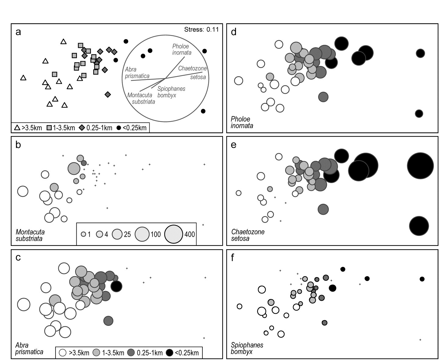
Fig. 7.13. Ekofisk oil-field macrofauna {E}. a) nMDS of 39 sites at different distances from the rig (a priori assigned to four distance groups, denoted by different symbols/shading), based on square-root transformed counts of 173 species and showing a clear gradient of community change with distance. Superimposed is a vector plot for five species, chosen to display a range of observed responses to the gradient, with the vector direction for each species reflecting the (Pearson) correlations of their (root-transformed) counts with the two ordination axes (the latter rotated, as usual for an MDS, to PCs), and length giving the multiple correlation coefficient from this linear regression on the ordination points (the circle is a correlation of 1). b-f) Individual bubble plots for these 5 species, on the same nMDS, with dot representing absence and circle sizes proportional to transformed counts; the back-transformed scale of original counts is in (b), common to all plots.
Fig. 7.13a replots the nMDS ordination of sediment macrofaunal assemblages (173 species) for 39 sites at different distances from the Ekofisk oil-field, in the form previously seen at Fig. 6.13a (based on square-root transformed counts). The a priori site groups at different distances are indicated by differing symbols but also by grey-shading, which is used in the bubble plots which follow, Figs. 7.13b-f, for five individual species. These are chosen to illustrate a range of the differing responses which meld together to produce the main gradient of assemblage change as sites near the oil-field (from four or five directions). That many species replicate each of these patterns, and more, is seen from the shade plot of Fig. 7.10b (that is based on log-transformed counts but the outcome is similar here). M. substriata is typical of species found in the background conditions but which are virtually absent at <1km from the oilrig. Species like A. prismatica are found in reasonable numbers right up to 250m from the rig but then appear to die out at the closest distances. P. inornata typifies an interesting group of species which, though present in background assemblages, are opportunists whose numbers increase as sites near the rig, in this case up to the very closest distances (<100m) before decreasing in abundance. C. setosa similarly shows an opportunist pattern with the highest counts in the matrix overall, and these are all within the <250m group, with counts increasing steadily as sites approach the oil-field centre. Counts of other species, such as S. bombyx, appear to bear a much weaker relation to the position of the points on the MDS, as well as having generally smaller values. Here, bubble sizes are chosen to be proportional to the transformed counts (and the common key, shown in b, back-transformed to original scales), in order to gauge relative species contributions to the MDS.
Vector plots
A great many bubble plots could be produced in this case, where the clear gradient is constructed from the combination of a large number of species, each highlighting particular parts of the gradient. It is therefore tempting to attempt to represent these in a single plot, each species defined by a vector whose direction and length define, respectively, the direction in the MDS space in which that species increases its counts, and the (multiple) correlation coefficient of that species with the ordination configuration†. The combination of these vectors is then superimposed on the MDS, as in Fig. 7.13a for the 5 species shown in the bubble plots of 7.13b-f. Technically, this is carried out by fitting multiple linear regression of the species counts to the MDS (x, y) co-ordinates – or (x, y, z) points if the MDS is in 3-d. If the MDS has been rotated such that the axes are uncorrelated (as noted earlier, this is automatic for the initial plot), then the vector lengths projected onto the x and y axes represent the Pearson correlations of that species with each axis. These are thus comparable across species in the vector diagram, with the circle representing a multiple correlation of 1, but note that since these are separate regressions for each species, differences in scale among species counts are not seen in vector lengths. They reflect (scale-free) correlations with axes, not contributions to the MDS, e.g. the smaller counts of S. bombyx, see Fig. 7.13f, do not of themselves shorten their vector.§
It is crucial to appreciate that the vector plot can be placed anywhere on the ordination plot, and can be scaled to any size, with its interpretation completely unchanged. This is often misunderstood, with users of vector plots sometimes inferring that the end point of a vector being close to a particular sample indicates, in some way, that this species takes its largest values at, or in the vicinity of, that sample. This is absolutely incorrect. All a vector indicates is a direction – the centre point of the vectors can be placed anywhere but the direction in which a vector extends from that point is the direction in which that variable increases, e.g. the lowest C. setosa values are expected to the left and highest to the right of the plot (as in 7.13e).
Widely used though such vector plots are, they have a serious problem, also poorly understood in the literature. They make the fundamental assumption that the relationship of species values to the plot co-ordinates is a linear one. But most of the bubble plots of Fig. 7.13 (and the much larger species set of Fig. 7.10b) do not show such a relationship. Here, only C. setosa displays a linear-like increase from left to right of the plot, and arguably S. bombyx (right to left), with a weaker correlation. Others are distinctly non-linear, M. substriata and A. prismatica having a threshold-type relation (constant then dropping to nothing), and P. inornata an increasing then decreasing pattern, not even monotonic. The telling comparison is between the vector plot of Fig. 7.13a and the bubble plots of b-f. Does the vector plot really describe the pattern of relationships seen in the bubble plots? Scarcely, when at all – it is unquestionably a poor substitute for them.
Nonetheless, a space limitation on multiple plots will often be encountered, and the ability to replace 4 or 5 bubble plots (or more) by a single graph is necessary. This may be achievable by segmented bubble plots.
Multi-variable (segmented) bubble plots
Fig. 7.14 condenses the bubble plots of Fig. 7.13b-e into a single MDS plot, by simply showing segments of a circle (or, in 3-d, a sphere), differently shaded or coloured, with sizes again reflecting values of those four species in each sample, also commonly scaled as before (root-transformed). Whilst colour would aid distinction of the species (which of course PRIMER allows), it is still possible to draw exactly the same inference from this graph as for the four bubble plots.
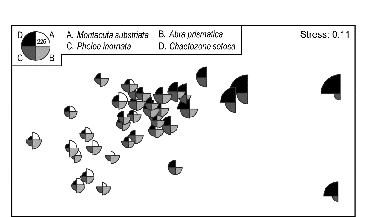
Fig. 7.14. Ekofisk oil-field macrofauna {E}. Segmented bubble plot for MDS ordination as in Fig. 7.13a, with segment sizes proportional to the root-transformed counts of four species, commonly scaled. The size of segments in the key corresponds to a count of 225, when back-transformed to the original scale.
A remarkably clear example of a similar graph is seen for the Bristol Channel zooplankton data last met in the shade plot of Fig. 7.8. This example uses the agglomerative clusters and MDS ordination of Fig. 3.10a, selecting four species to display by the criterion that they head the list of typifying species for each of the four clusters in the corresponding SIMPER analysis table‡. The combination of information from a shade plot and SIMPER analyses will often dictate species which could be usefully graphed in this way. Note that the bubble segment sizes use the original scales here and not the fourth-root transformed values that went into the MDS construction. This is a legitimate and often useful step, if the requirement is primarily to look at how the abundance of individual species behaves, e.g. over a community gradient, rather than the precise influence this has on the MDS itself. In that context, separate scaling of variables is not only permissible, it is almost mandatory if the plot is to be interpretable, e.g. here the Eurytemora values range only up to <500 whereas the maximum Paracalanus density is >30,000 (this is precisely why a severe 4th-root transform was essential in this case, of course). We shall also see later (Chapter 11) that bubble plots have a useful role in displaying environmental-type variables on the points of an assemblage ordination, and the original units are rarely commonly scalable.
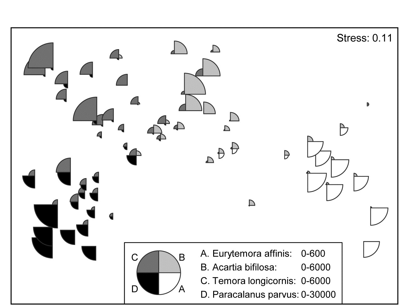
Fig. 7.15. Bristol Channel zooplankton {B}. Segmented bubble plot on nMDS ordination of the 57 sites, using Bray-Curtis on $\sqrt{} \sqrt{}$- abundances, leading by Type 1 SIMPROF to the 4 site clusters (A-D) of Fig. 3.10a, agglomerative clustering. Bubble segments are proportional to raw counts of the four species which ‘most typify’ those clusters, from SIMPER tables. Counts for these species (correspondingly labelled A-D) are differently scaled.
Segmented bubble plots often prove most useful when the number of points on an ordination plot is small and the sampling error of each point has been substantially reduced, so that the picture consists mainly of genuine differences; then it is sometimes possible to show quite large numbers of species simultaneously. Such bubble plots thus have a strong role to play in means plots.
Example: W Australian fish diets
Hourston, Platell, Valesini et al. (2004) and Schafer, Platell, Valesini et al. (2002) report dietary data on gut contents (identified to one of 32 taxon groups) of 7 marine fish species in nearshore, lower west coast Australian waters. Analysis was of sample-standardised (thus percent composition) data, in similar fashion to that for the (different) labrid fish dietary data of Fig. 16.5. The nMDS plot⸙ of Fig. 7.16 is based on meaned data over all fish guts for each of the 7 species (species names shown on the plot). This time it is SIMPER tables of the major dietary contributors, to the dissimilarities between fish species pairs, which have identified 6 dietary taxon groups to show as segmented bubbles overlaid on the mean points. Interpretation of the differing dietary regimes found amongst these co-occurring species, including those for three congeneric species, is now clear and direct, but must of course be made in conjunction with tests (such as in ANOSIM or PERMANOVA) to establish their statistical significance.
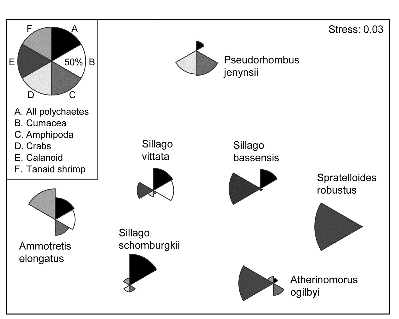
Fig. 7.16. Diets of W Australian fish {d}. Segmented bubble plot. nMDS ordination (using Bray-Curtis similarities) of standardised, transformed, then averaged gut compositions (by volume) of 32 broad dietary categories, from 7 abundant fish species in nearshore habitats. Superimposed bubble segment sizes represent % composition (untransformed) for 6 dietary categories, shown from SIMPER analysis to contribute most to the average dissimilarities among the diets of the different fish species. Segment sizes are commonly scaled here (key sizes represent 50% composition).
¶ PRIMER can plot 3-d versions (when the term ‘bubble plot’ is more appropriate!) for both simple and segmented bubble plots, though none are reproduced here since rotatable 3-d colour plots are not very successfully reproduced in static 2-d mono pictures.
† Significance tests for these correlations would not be valid, not least because the vectors represent species which are part of the full set used to create the ordination points in the first place!
§ There are two other definitions of vectors available in PRIMER for 2- or 3-d ordinations. Pearson, here, is the default; an alternative is a multivariate (multiple) correlation method, which fits the supplied superimposed variables jointly, so vector directions will change if further variables are added, see discussion in the PERMANOVA+ manual, Anderson, Gorley & Clarke (2008) , where this is used with Principal Co-ordinates, PCO. A third method (‘base variables’) arises only for PCA plots, a relevant ordination for analysis of environmental-type data, not the current case. The vectors then reflect the relative size and magnitude of coefficients of each variable in the PC1, PC2,... definitions, as in equation (4.1). Linear relationships of these variables to the co-ordinates of the plot is thus guaranteed and a vector plot always justified.
‡ Of the type seen in Table 7.2, noting that Eurytemora affinis will head this table if the agglomerative groups are used (page 7.8).
⸙ As seen on page 5.9, nMDS plots with few points, as here, can collapse, e.g. because one species predates on primarily different dietary categories than found anywhere else in the matrix. Metric MDS (or an nMDS solution which mixes a small amount of metric stress, to ‘fix’ the collapse) are often useful for such means plots, though they were not necessary in this case, with the main dietary categories usually being shared between more than one species.