6.15 Example: King Wrasse fish diets, WA
We begin the 3-factor examples with a fully crossed design A$\times$B$\times$C of the composition by volume of the taxa found in the foreguts of King Wrasse fish from two regions of the western Australian coast, just part of the data on labrid diets studied by Lek, Fairclough, Platell et al. (2011) , {k}. Taxonomic composition of the prey assemblage was reduced to 21 broad groups (such as gastropods, bivalves, annelids, ophiuroids, echinoids, small and large crustaceans, teleost fish, etc). Here the fish are ‘doing the sampling’ of the assemblages and there is, naturally, no control over the total volume of material in each gut, so standardisation of the taxon volumes to relative composition (all taxa add to 100% for each sample) is essential. In addition, prior to this, foregut contents of c. 4 fish need to be (randomly) pooled to make a viable single sample of ingested material.
For this illustration, the base-level samples have been further pooled to give two replicate times from each combination of A: three region/habitat levels (Jurien Bay Marine Park, JBMP, at exposed and sheltered sites, and Perth coast exposed sites); B: body size of the wrasse predator, with four ordered levels; C: two seasonal periods, summer/autumn and winter/spring¶.
Three-factor crossed ANOSIM (case 3c in Table 6.4, but for B ordered rather than C), testing for A within all 8 combinations of B and C levels gives $\overline{R} = 0.26$ ($p \approx$ 1.5%, on a random subset of 9999 from the $15^8$ possible permutations); the pairwise tests between the region/habitat levels (now on $3^8 = 6561$ permutations) give similar values of $\overline{R}$ between 0.20 and 0.29. The ordered ANOSIM test for length-class B, across the 6 strata of A and C, has a larger $\overline{R}^{Oc}$ of 0.49 (p<0.01%) with a clear pattern in the pairwise $\overline{R}$ of increasing values with wider-separated wrasse size-classes ($R_{12}$, $R_{23}$, $R_{34}$ = 0, 0.21, 0.08; $R_{13}$, $R_{24}$ = 0.46, 0.5; $R_{14}$ = 0.63; p<5% only for the last three tests). Unsurprisingly therefore, the appropriately ordered ANOSIM test outperforms the equivalent unordered test (case 3a), which has $\overline{R} = 0.32 $ (p<0.1%). The test for period C, removing A and B, gives no effect, with $\overline{R} = 0.0$.
The key point here is that the 3 global statistics, $\overline{R}$ or $\overline{R}^{Oc}$ of A: 0.26, B: 0.49, C: 0 (and pairwise values), are directly comparable as measures of the effect size for each factor; the ANOSIM statistic is not hi-jacked by the differences in group sizes, in sharp contrast to the significance level, p, which never escapes strong dependence on the number of permutations.
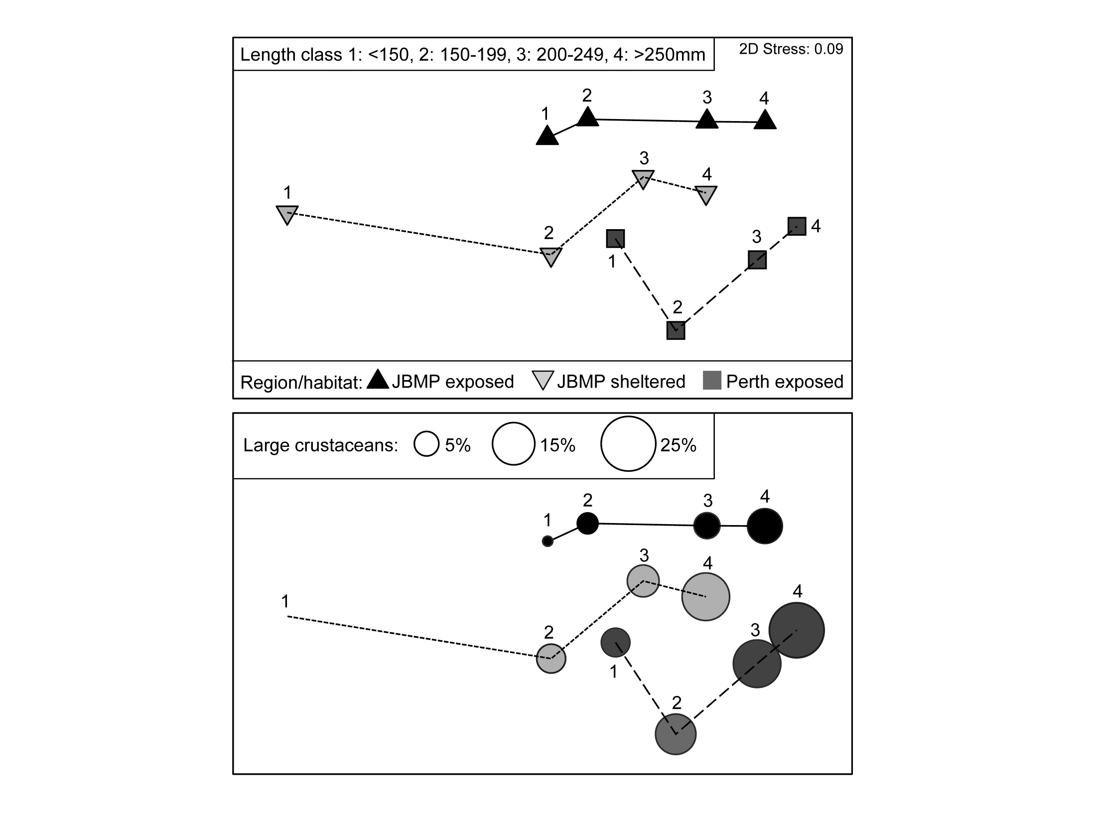 Fig. 6.15. King Wrasse diets {k}. nMDS (on Bray-Curtis) of $\sqrt{}$ taxon volumes averaged over replicates and seasonal periods, showing clear dietary change with King Wrasse body size and between regions/habitats; lower plot overlays bubbles with sizes proportional to one component of the average diet.
As for univariate ANOVA, the natural successor to hypothesis tests should be a means plot, illustrating these effect sizes. Since the period effect is absent, an average of the data matrix over both the 2 replicates and 2 periods is appropriate†. The resulting nMDS of the dietary assemblages for the 4 wrasse size-classes at the 3 locations is shown in Fig. 6.15. It has low stress (0.09) and displays the relationships seen in the tests with great clarity, unlike the high-stress (0.19) nMDS on the full set of samples, which is the typical ‘blob’ of replicate-level plots (an often useful mantra is: ‘test on the replicates – but ordinate the means’!).
The next question is always likely to be: ‘and which taxa are mainly implicated in the steady change in the dietary assemblage through the size classes?’. This is the subject of Chapter 7, but one of the simplest and most effective tools is a bubble plot, superimposing on each ordination point a circle (or in 3-d, a sphere) with size proportional to the (averaged) value for a specific taxon in that (averaged) sample. The lower plot in Fig. 6.15 shows a bubble plot for the ‘large crustaceans’, which are seen to become an increasing part of King Wrasse diet with size, in all locations.
¶ The original data potentially have a 5-factor crossed design, treating region and habitat separately and with 2 further common labrid species studied, but such higher-way designs can always be analysed at a lower level, flattening pairs of factors, as for A above. In fact, Lek, Fairclough, Platell et al. (2011) found it necessary to analyse only 3 factors at a time to explore dietary change with region, habitat, species, size and season because there were no sheltered sites on the Perth coast, and not all labrid species and not all size classes were found in each location. Examining different hypotheses may often require separate analysis of different selections from a data set, and you should not be reluctant to do this!
† Average the transformed data not the original matrix, or use the ‘distances among centroids’ option in PERMANOVA+, though again these give virtually identical plots, see footnote on page 5.9. The major step forward that PERMANOVA takes, albeit under the more restrictive assumptions of a linear model, is that it allows partitioning of the effects seen here into ‘main effects’ and ‘interactions’, something which is simply undefinable in a non-parametric approach (see later). Here, PERMANOVA tests give no evidence at all for any interactions: as the ordination shows, the orderly progression of diet as the wrasse grows is maintained in much the same way across the differing conditions (balance of food availability, in part, presumably) at the three locations.