17.11 Taxonomic dissimilarity
A natural extension of the ideas of this chapter is from $\alpha$- or ‘spot’ diversity indices to $\beta$- or ‘turn-over’ diversity. The latter are essentially based on measures of dissimilarity between pairs of samples, the starting point for most of the methods of this manual. It is intriguing to ask whether there are natural analogues of some of the widely-used ‘biological’ dissimilarity coefficients, such as Sørensen (Bray-Curtis on presence/absence data, equation 2.7) or Kulczynski (P/A, equation 2.8), which exploit the taxonomic, phylogenetic or genetic relatedness of the species making up the pair of samples being compared. Thus two samples would be considered highly similar if they contain the same species, or closely related ones, and highly dissimilar if most of the species in one sample have no near relations in the other sample.
In fact, Clarke & Warwick (1998a) first defined a taxonomic mapping similarity between two species lists, in order to examine the taxonomic relatedness of the species sets successively ‘peeled’ from the full list, in a structural redundancy analysis of influential groups of species (the M statistic of Chapter 16, Table 16.2). This turns out to be the natural extension of Kulczynski dissimilarity and (to be consistent with our use in Chapter 17 of u.c. Greek characters for taxonomic relatedness measures) it is denoted here by $\Theta ^ +$. Izsak & Price (2001) used a slightly different form of coefficient, which proves to be the extension of the Sørensen coefficient, denoted here by $\Gamma ^ +$. Before defining these coefficients, however, it is desirable to state the potential benefits of such a taxonomic dissimilarity measure:
a) samples from different biogeographic regions do not lend themselves to conventional clustering or MDS ordination analyses using Sørensen (Bray-Curtis) or other traditional similarity coefficients. This is because few species may be shared between samples from different parts of the world. In extreme cases, there may be no species in common among any of the samples and all Bray-Curtis dissimilarities will be 100, leaving no possibility for a dendrogram or ordination plot. A taxonomic dissimilarity measure, however, takes into account not just whether the second sample has matching species to the first sample but, if it does not, whether there are closely related species in the second sample to all those found in the first sample (and vice-versa). Two lists with no species in common therefore have a defined dissimilarity, measuring whether they contain distantly or closely related species, and meaningful MDS plots ensue.
b) standard similarity measures will, inevitably, be susceptible to variation in taxonomic expertise or (in the case of time series) revisions in taxonomic definition, across the samples being compared. For example, suppose at some point in a time series, an increase in taxonomic expertise results in what was previously identified as a single taxon being noted as two separate species. The data should, of course, be subsequently rationalised to the lowest common denominator of taxonomic identification over the full series, but if this is not done, an ordination will have a tendency to display some artefactual signal of ‘community change’ at this point (one species has disappeared and two new ones have appeared). A single occurrence of this sort will not have much effect – one of the advantages of similarities based on presence/absence data is that they draw only a little information from each species – but if taxonomic inconsistency is rampant, misleading ordinations could result. Taxonomic dissimilarity would, however, be more robust to species being split in this way. The later samples do not appear to have the same taxon as the earlier samples, but they have one (or two) species which are very closely related to it (the same genus), hence retain high contributions to similarity from that species.
c) it might be hoped that the desirable sampling properties of taxonomic distinctness indices such as $\Delta ^ +$ and $\Lambda ^ +$, in particular their robustness to variable sampling effort across the samples, would carry over to taxonomic dissimilarity measures.
Taxonomic dissimilarity definition
As in Table 16.2, the distance through the taxonomic, (or phylogenetic/genetic) hierarchy, from every species in the first sample (A) to its nearest relation in the second sample (B), is recorded. These are totalled, as are the distances between species in sample B and their nearest neighbours in sample A, see the example in Fig. 17.18. These two totals are not the same, in general, and the way they are converted to an average taxonomic distance between the two samples defines the difference between $\Gamma ^ +$ and $\Theta ^ +$. Formally, if $\omega _ {ij}$ is the path length between species i and j, and there are $s _ A$ and $s _ B$ species in samples A and B, then:
$$\Gamma ^ + = 100 \times \left( \sum _ {i \in A} \min _ {j \in B} ( \omega _ {ij} ) + \sum _ {j \in B} \min _ {i \in A} ( \omega _ {ji}) \right) \big/ (s _ A + s _ B)$$ $$\Theta ^ + = 100 \times \frac{1}{2} \left( \frac{ \sum _ {i \in A} \min _ {j \in B} ( \omega _ {ij} )}{s _A} + \frac{ \sum _ {j \in B} \min _ {i \in A} ( \omega _ {ji})}{s _B} \right) \tag{17.8}$$
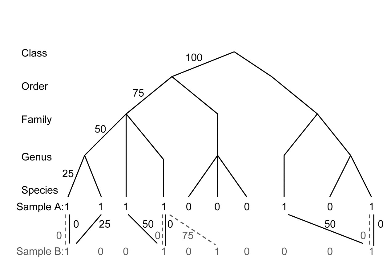
Fig. 17.18. For presence/absences from two hypothetical samples (A with 6 species, B with four), distances through the tree from each species in A to its nearest neighbour in B (black, continuous join) and vice-versa (grey, dashed join).
In words, $\Gamma ^ +$ is the average path length to the nearest relation in the opposite sample¶, i.e. a simple average of all the path lengths shown in Fig. 17.18. Thus:
$$\Gamma ^ + = [(0+25+50+0+50+0)+(0+0+75+0)]/(6+4) = 20.0 $$
whereas $\Theta ^ +$ is a simple mean of the separate averages in the two directions: A to B, then B to A. Thus:
$$\Theta ^ + = [(125/6) + (75/4)]/2 = 19.8 $$
Clearly, the two measures give identical answers if the number of species is the same in the two samples, and they cannot give very different dissimilarities unless the richness is highly unbalanced. This is precisely as found for the relationship between the Bray-Curtis and Kulczynski measures on P/A data; they cannot give a different ordination plot unless species numbers are very variable. The relation of these standard coefficients to $\Gamma ^ +$ and $\Theta ^ +$ is readily seen: imagine flattening the taxonomic hierarchy to just two levels, species and genus, with all species in the same genus, so that different species are always 100 units apart. The branch length between a species in sample A and its nearest neighbour in sample B is either 0 (the same species is in sample B) or 100 (that species is not found in sample B). In that case:
$$\Gamma ^ + = (300 + 100)/(6+4) = 40.0 \equiv B ^ + $$ $$ \Theta ^ + = (300/6 + 100/4)/2 = 37.5 \equiv K ^ + \tag{17.8}$$
where $B ^ +$ and $K ^ +$ denote Bray-Curtis and Kulczynski dissimilarity for P/A data, respectively. The truth of this identity can be seen from their general definitions (see equations 2.7 and 2.8 for the similarity forms):
$$ B ^ + = (100 b + 100 c)/[(a + b) + (a + c)] $$ $$ K ^ + = [(100 b)/(a + b) + (100 c) / (a + c)]/2 \tag{17.9} $$
where b is the number of species present in sample A but not sample B, c is the number present in B but not A, and a is the number present in both. Clearly, 100b is the total of the (a+b) path lengths from A to B, and 100c the total of the (a+c) path lengths from B to A.
Taxonomic dissimilarity, $\Gamma ^ +$, is therefore a natural generalisation of the Sørensen coefficient, adding a more graded hierarchy on top of standard Bray-Curtis (instead of matching ‘hits’ and ‘misses’ there are now ‘near hits’ and ‘far misses’). In some ways, this is analogous to the relationship shown earlier, between Simpson diversity ($\Delta ^ \circ$) and taxonomic diversity ($\Delta$), and it has two likely consequences:
-
ordinations based on $\Gamma ^ +$ will bear an evolutionary, rather than revolutionary, relationship to those based on P/A Bray-Curtis†; when there are many direct species matches $\Gamma ^ +$ may tend to track B$^ +$ rather closely.
-
$\Gamma ^ +$ will tend to carry across the sampling properties of B$^ +$; it is well-known that Bray-Curtis (and indeed, all widely-used dissimilarity coefficients) are susceptible to bias from variations in sampling effort. It is axiomatic in multivariate analysis that similarities be calculated between samples which are either rigidly controlled to represent the same degree of sampling effort, or in the case of non-quantitative sampling, samples are large enough for richness to be near the asymptote of the species -area curve (this is very difficult to arrange in most practical contexts!) Otherwise, it is inevitable that samples of smaller extent will contain fewer species and thus similarities calculated with larger samples will be lower, even when true assemblages are the same. Theory shows that, indeed, $\Gamma ^ +$ and $\Theta ^ +$ (along with B$^ +$, K$ ^ +$, $\Phi ^ +$) are not independent of sampling effort, so the third of our hoped-for properties for taxonomic dissimilarity – that it would carry across the nice statistical properties of taxonomic distinctness measures $\Delta ^ +$ and $\Lambda ^ +$ – is not borne out§.
The other two potential advantages of taxonomic dissimilarity, given above, do stand up to practical examination. One of us (PJS), in the description of these taxonomic dissimilarity measures in Clarke, Somerfield & Chapman (2006) , gives the following two examples.
¶ $\Gamma ^ +$ is the taxonomic distance, ‘TD’, of Izsak & Price (2001) (not to be confused with the AvTD and TTD of this chapter, which are diversity indices not dissimilarities!), except that the longest path length in their taxonomic trees is not scaled to a fixed number, such as 100 or 1, so they rescale it in similarity form, denoted $\Delta _s$.
† It is tempting to define, by analogy with equations (17.1) to (17.3), a further coefficient, the ratio $\Phi ^ + = \Gamma ^ + / B ^ +$, which reflects more purely the relatedness dissimilarity, removing the Bray-Curtis component in $\Gamma ^ +$, coming from direct species matches. In fact, $\Phi ^ +$ is simply the average of the minimum distance from each species to its nearest relation in the other sample, calculated only for the ‘b+c’ species which do not have a direct match. It is thus independent of ‘a’ (number of matches) as well as ‘d’ of course (number of joint absences). Limited practical experience, however, suggests that $\Phi ^ +$ tends to ‘throw the baby out with the bathwater’ and leads to uninterpretably ‘noisy’ ordination plots.
§ Note, however, that Izsak & Price (2001) provide some limited simulation evidence for $\Gamma ^ +$ being less biased by uneven sampling effort than one of the other standard P/A indices, Jaccard, equation (2.6). This suggests that the comparison with Sørensen – the more natural comparator, given the above discussion – would also indicate some advantage for the taxonomic dissimilarity measure (Jaccard and Sørensen are quite closely linked, in fact monotonically related, so they produce identical non-metric MDS plots for example).