3.5 Similarity profiles (SIMPROF)

Given the form of the dendrogram in Fig. 3.3, with high similarities in apparently tightly defined groups and low similarities among groups, there can be little doubt that some genuine clustering of the samples exists for this data set. However, a statistical demonstration of this would be helpful, and it is much less clear, for example, that we have licence to interpret the sub-structure within any of the four apparent main groups. The purpose of the SIMPROF test is thus, for a given set of samples, to test the hypothesis that within that set there is no genuine evidence of multivariate structure (and though SIMPROF is primarily used in clustering contexts, multivariate structure could include seriation of samples, as seen in Chapter 10). Failure to reject this ‘null’ hypothesis debars us from further examination, e.g. for finer-level clusters, and is a useful safeguard to over-interpretation. Thus, here, the SIMPROF test is used successively on the nodes of a dendrogram, from the top downwards.

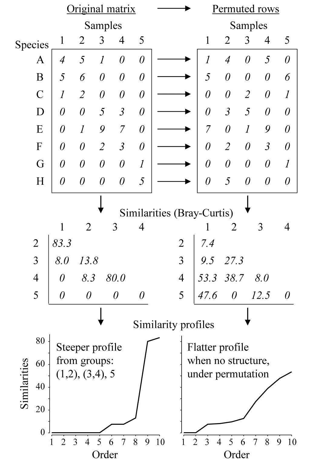Fig. 3.4. Simple example of construction of a similarity profile from 5 samples (1-5) of 8 species (A-H), for the original matrix (left-hand column) and in a permuted form (right-hand column).
 

Construction of a single SIMPROF test

The SIMPROF technique is based on the realisation that there is a duality between structure in samples and correlation (association) in species, and Fig. 3.4 demonstrates this for a simple example. The original matrix, in the left-hand column, appears to have a structure of three clusters (samples 1 and 2, samples 3 and 4, and sample 5), driven by, or driving, species sets with high internal associations (A-C, D-F and G-H). This results in some high similarities within the clusters (80, 83.3) and low similarities between the clusters (0, 8, 8.3, 13.8) and few intermediate similarities, in this case none at all. Here, the Bray-Curtis coefficient is used but the argument applies equally to other appropriate resemblance measures. When the triangular similarity matrix is unravelled and the full set of similarities ordered from smallest to largest and plotted on the y axis against that order (the numbers 1, 2, 3, …) on the x axis, a relatively steep similarity profile is therefore obtained (bottom left of Fig. 3.4).

In contrast, when there are no positive or negative associations amongst species, there is no genuinely multivariate structure in the samples and no basis for clustering the samples into groups (or, indeed, identifying other multivariate structures such as gradients of species turnover). This is illustrated in the right-hand column of Fig. 3.4, where the counts for each row of the matrix have been randomly permuted over the 5 samples, independently for each species. There can now be no genuine association amongst species – we have destroyed it by the randomisation – and the similarities in the triangular matrix will now tend to be all rather more intermediate, for example there are no really high similarities and many fewer zeros. This is seen in the corresponding similarity profile which, though it must always increase from left to right, as the similarities are placed in increasing order, is a relatively flatter curve (bottom right, Fig. 3.4).

This illustration suggests the basis for an effective test of multivariate structure within a given group of samples: a schematic of the stages in the SIMPROF permutation test is shown in Fig. 3.5, for a group of 7 samples. The similarity profile for the real matrix needs to be compared with a large set of profiles that would be expected to occur under the null hypothesis that there is no multivariate structure in that group. Examples of the latter are generated by permutation: the independent random re-arrangement of values within rows of the matrix, illustrated once in Fig. 3.4, is repeated (say) 1000 times, each time calculating the full set of similarities and their similarity profile. The bundle of ‘random’ profiles that result are shown in Fig. 3.5 by their mean profile (light, continuous line) and their 99% limits (dashed line). The latter are defined as intervals such that, at each point on the x axis, only 5 of the 1000 permuted profiles fall above, and 5 below, the dashed line. Under the null hypothesis, the real profile (bold line) should appear no different than the other 1000 profiles calculated. Fig. 3.5 illustrates a profile which is not at all in keeping with the randomised profiles and should lead to the null hypothesis being rejected, i.e. providing strong evidence for meaningful clustering (or other multivariate structure) within these 7 samples.

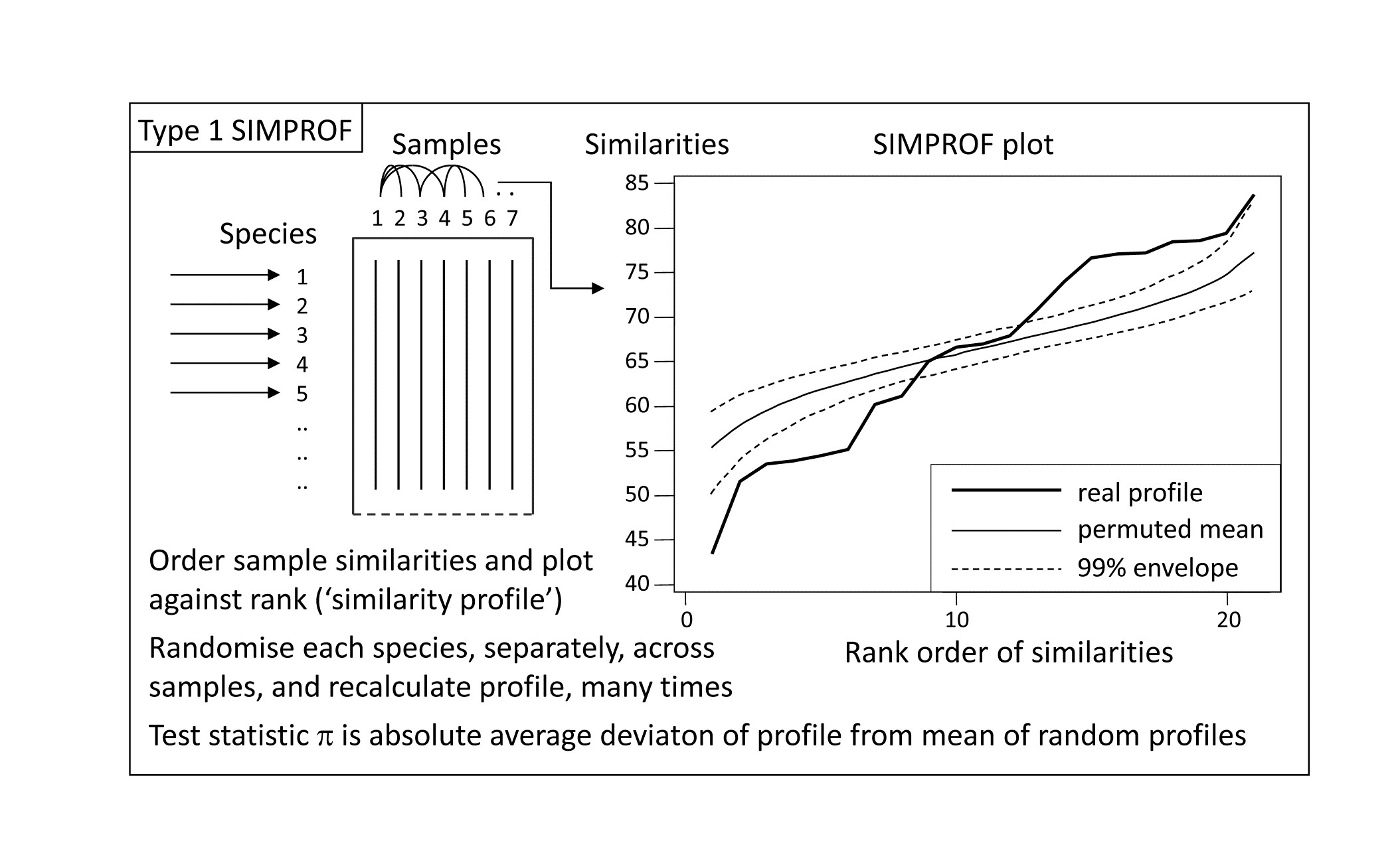Fig. 3.5. Schematic diagram of construction of similarity profile (SIMPROF) and testing of null hypothesis of no multivariate structure in a group of samples, by permuting species values. (This is referred to as a Type 1 SIMPROF test, if it needs to be distinguished from Type 2 and 3 tests of species similarities – see Chapter 7. If no Type is mentioned, Type 1 is assumed). *

 

A formal test requires definition of a test statistic and SIMPROF uses the average absolute departure $\pi$ of the real profile from the mean of the permuted ones (i.e. positive and negative deviations are all counted as positive). The null distribution for p is created by calculating its value for 999 (say) further random permutations of the original matrix, comparing those random profiles to the mean from the original set of 1000. There are therefore 1000 values of $\pi$, of which 999 represent the null hypothesis conditions and one is for the real profile. If the real $\pi$ is larger than any of the 999 random ones, as would certainly be the case in the schematic of Fig. 3.4, the null hypothesis could be rejected at least at the p < 0.1% significance level. In less clear-cut cases, the % significance level is calculated as 100(t+1)/(T+1)%, where t of the T permuted values of $\pi$ are greater than or equal to the observed $\pi$. For example, if not more than 49 of the 999 randomised values exceed or equal the real $\pi$ then the hypothesis of no structure can be rejected at the 5% level.*
 

SIMPROF for Bristol Channel zooplankton data

Though a SIMPROF test could be used in isolation, e.g. on all samples as justification for starting a multivariate analysis at all, its main use is for a sequence of tests on a hierarchical group structure established by an agglomerative (or divisive) cluster analysis. Using the Bristol Channel zooplankton dendrogram (Fig. 3.3) as an illustration, the first SIMPROF test would be on all 57 sites, to establish that there are at least some interpretable clusters within these. The similarity profile diagram and the resulting histogram of the null distribution for $\pi$ are given in the two left-hand plots of Fig. 3.6. Among the $(57 \times 56)/2 = 1596$ similarities, there are clearly many more large and small, and fewer mid-range ones, than is compatible with a hypothesis of no structure in these samples. (Note that the large number of similarities ensures that the 99% limits hug the mean of the random profiles rather closely.) The real $\pi$ of 6.4 is seen to be so far from the null distribution as to be significant at any specified level, effectively.

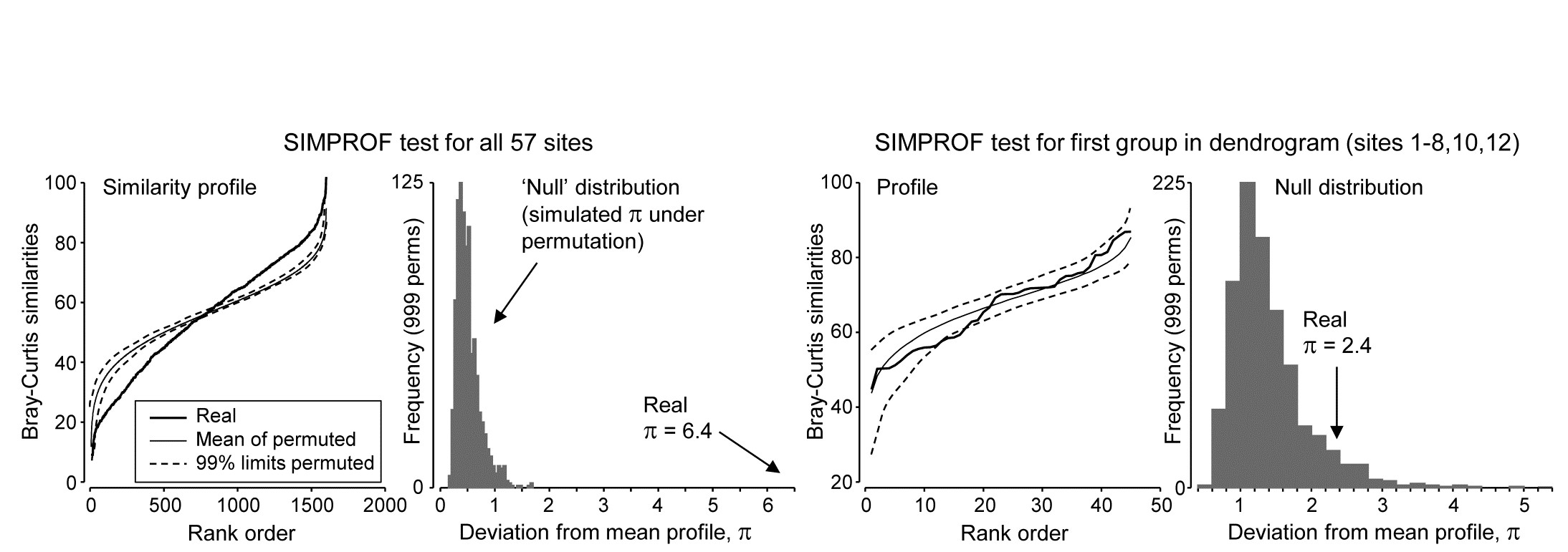
Fig. 3.6. Bristol Channel zooplankton {B}. Similarity profiles and the corresponding histogram for the SIMPROF test, in the case of (left pair) all 57 sites and (right pair) the first group of 10 sites identified in the dendrogram of Fig. 3.3 *
 

As is demonstrated in Fig. 3.7, we now drop to the next two levels in the dendrogram. On the left, what evidence is there now for clustering structure within the group of samples {1-8,10,12}? This SIMPROF test is shown in the two right-hand plots of Fig. 3.6: here the real profile lies within the 99% limits over most of its length and, more importantly, the real $\pi$ of 2.4 falls within the null distribution (though in its right tail), giving a significance level p of about 7%. This is marginal, and would not normally be treated as evidence to reject the null hypothesis, especially bearing in mind that multiple significance tests are being carried out.

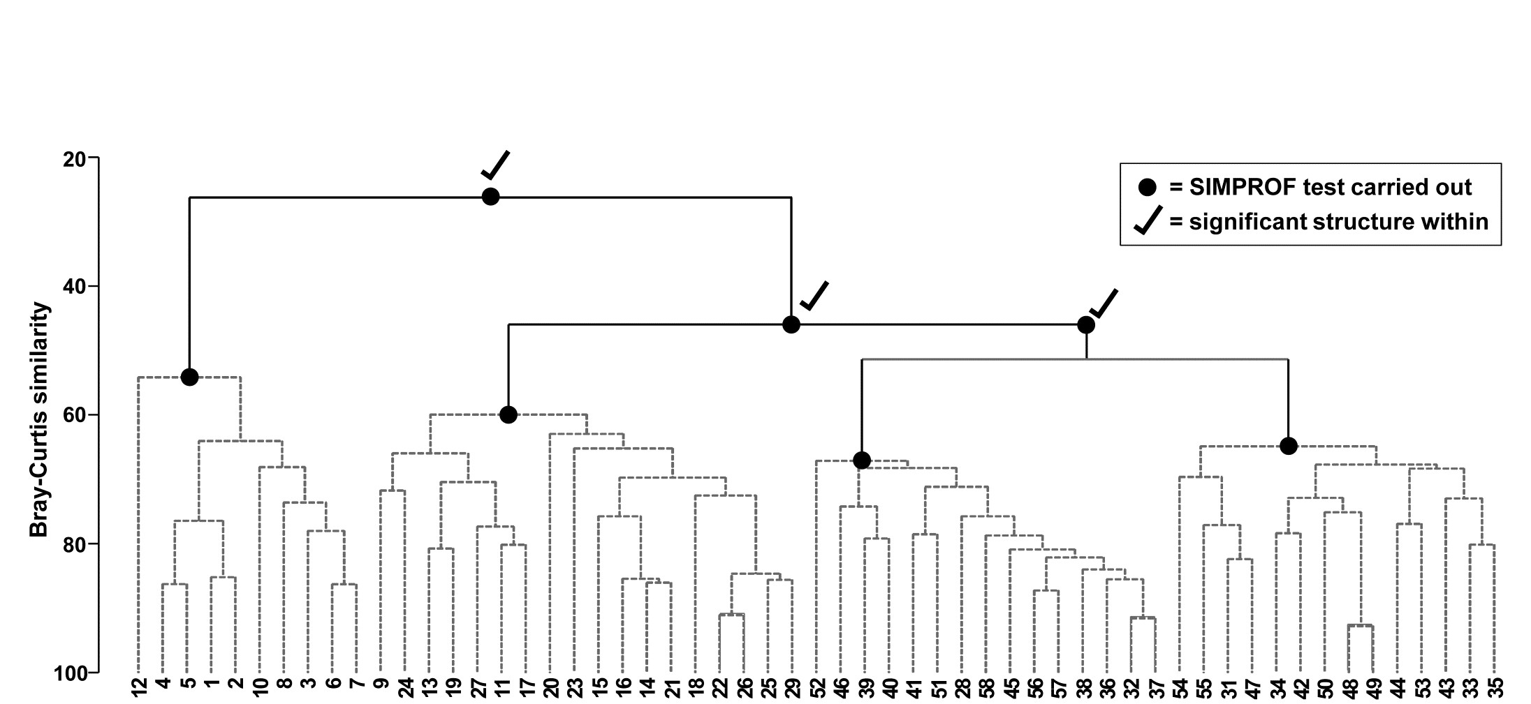
Fig. 3.7. Bristol Channel zooplankton {B}. Dendrogram as in Fig. 3.4 but showing the results of successive SIMPROF tests on nodes of the tree, starting at the top. Only the first three tests showed significant multivariate structure in the samples below that point (bold dots), so there is no evidence from SIMPROF for the detailed clustering structure (grey dashed lines) within each of the 4 main groups.
 

The conclusion is therefore that there is no clear evidence to allow interpretation of further clusters within the group of samples 1-8,10,12 and this is considered a homogenous set. The remaining 47 samples show strong evidence of heterogeneity in their SIMPROF test (not shown, $\pi = 3.4$, way off the top of the null distribution), so the process drops through to the next level of the dendrogram, where the left-hand group is deemed homogeneous and the right hand group again splits, and so on. The procedure stops quickly in this case, with only four main groups identified as significantly different from each other. The sub-structure of clusters within the four main groups, produced by the hierarchical procedure, therefore has no statistical support and is shown in grey dashed lines in Fig 3.7.
 

Features of the SIMPROF test

These are discussed more extensively in the primary paper on SIMPROF, , but some important attributes of the test are worth noting here.

1. A key feature of permutation tests, which are exploited many times in this manual, is that the distribution of abundances (or biomass, area cover etc) for each species remains exactly the same under the random permutations, and is therefore fully realistic. Some species are highly abundant whilst some are much rarer, some species have very right-skewed values, some much less so, and so on. All of this is represented faithfully in the permuted values for each species, since they are exactly the same counts. There is no need to assume specific probability distributions for the test statistics (as in classic statistical tests) or to invoke particular probability distributions for the observations, from which to create matrices simulating the original data (as in Monte Carlo testing). The original data is simply re-used, but in a way that is consistent with the null hypothesis being tested. This makes permutation tests, for hypotheses where they can be exploited, extraordinarily general and powerful, as well as simple to understand and interpret.
    

2. There are at least two asymmetries in the interpretation of a sequence of SIMPROF tests from a cluster hierarchy. Firstly, they provide a ‘stopping rule’ for how far down a dendrogram structure may be interpreted which is not a constant similarity ‘slice’ over the hierarchy: some branches may contain more samples exhibiting more detailed structure, which is validly interpretable at higher similarity levels than other branches. Secondly, in cases where the test sequence justifies interpreting a rather fine-scale group structure (which it would therefore be unwise to interpret at an even more detailed level), it may still be perfectly sensible to choose a coarser sample grouping, by slicing at a lower similarity. SIMPROF gives limits to detailed interpretation but the groups it can identify as differing statistically may be too trivially different to be operationally useful.
    

3. There can be a good deal of multiple testing in a sequence of SIMPROF tests. Some adjustment for this could be made by Bonferroni corrections. Thus, for the dendrogram of Fig. 3.7, a total of 7 tests are performed. This might suggest repeating the process with individual significance levels of 5/7 = 0.7%, but that is over-precise. What would be informative is to re-run the SIMPROF sequence with a range of significance levels (say 5%, 1%, 0.1%), to see how stable the final grouping is to choice of level. (But scale up your numbers of permutations at higher significance levels, e.g. use at least 9999 for 0.1% level tests; 999 would simply fail to find any significance!). In fact, you are highly likely to find that tinkering with the precise significance levels makes little difference to such a sequence of tests; only a small percentage of the cases will be borderline, the rest being clear-cut in one or other direction. In Fig. 3.7 for example, all four groups are maintained at more stringent significance levels than 5%, until unreasonable levels of 0.01% are reached, when the third and fourth groups (right side of plot) merge.
    

4. The discussion of more stringent p values naturally raises the issue of power of SIMPROF tests. Power is a difficult concept to formalise in a multivariate context since it requires a precise definition of the alternative to the null hypothesis here of ‘no multivariate structure’, when in fact there are an infinite number of viable alternatives. (These issues are mentioned again in Chapters 6 and 10, and see also Somerfield, Clarke & Olsgard (2002) ). However, in a general sense it is plausible that, all else being equal, SIMPROF will be increasingly likely to detect structure in a group of samples as the group size increases. This is evident if only from the case of just two samples: all random and independent permutations of the species entries over those two samples will lead to exactly the same similarity, hence the real similarity profile (a point) will be at the same position as all the random profiles and could never lead to rejection of the null hypothesis – groups of two are never split. Surprisingly often, though, there is enough evidence to split groups of three into a singleton and pair, an example being for samples 3, 4 and 5 of Fig. 3.4.
    

5. The number of species will also (and perhaps more clearly) contribute to the power of the test, as can be seen from the obvious fact that if there is just one species, the test has no power at all to identify clusters (or any other structure) among the samples. It does not work by exploring the spacing of samples along a single axis, for example to infer the presence of mixture distributions, a process highly sensitive to distributional assumptions. Instead, it robustly (without such assumptions) exploits associations among species to infer sample structure (as seen in Fig 3.3), and it seems clear that greater numbers of species should give greater power to that inference. It might therefore be thought that adding a rather unimportant (low abundance, low presence) species to the list, highly associated with an existing taxon, will automatically generate significant sample structure, hence of little practical consequence. But that is to miss the subtlety of the SIMPROF test statistic here. It is not constructed from similarities (associations) among species but sample similarities, which will reflect only those species which have sufficient presence or abundance to impact on those similarity calculations (under whatever pre-treatment options of standardising or transforming samples has been chosen as relevant to the context). In other words, for a priori unstructured samples, the test exploits only species associations (either intrinsic or driven by differing environments) that matter to the definition of community patterns, and it is precisely the presence of such associations that define meaningful assemblage structure in that case.

One final point to emphasise. It will be clear to those already familiar with the ANOSIM and RELATE tests of Chapters 6 and 10 that SIMPROF is a very different type of permutation test. ANOSIM starts from a known a priori structure of groups of samples (different sites, times, treatments etc, as in Fig. 3.1), containing replicate samples of each group, and tests for evidence that this imposed group structure is reflected in real differences in similarities calculated among and within groups. If there is such an a priori structure then it is best utilised: though SIMPROF is not invalid in this case, the non-parametric ANOSIM test, or the semi-parametric PERMANOVA test (see the Anderson, Gorley & Clarke (2008) manual) are the correct and better tests. If there is no such prior structuring of samples into groups, and the idea is to provide some rigour to the exploratory nature of cluster analysis, then a sequence of SIMPROF tests is likely to be an appropriate choice: ANOSIM would definitely be invalid in this case. Defining groups by a cluster analysis and then using the same data to test those groups by ANOSIM, as if they were a priori defined, is one of the most heinous crimes in the misuse of PRIMER, occasionally encountered in the literature!