8.5 Multivariate tools used on univariate data
Ekofisk macrofauna: testing dominance curves
Fig. 8.5b compares the averaged community samples for the closest distances to the oil platform (< 250m) with the second closest group (250m – 1km), in terms of their k-dominance curves, and the closest samples appear to be more heavily dominated. But, to test this, we must return to the replicate rather than averaged curves, and these are seen for the 6 and 10 samples in the two distance groups in Fig. 8.14a,b, the two plots being identical apart from a log scaled x axis in (a).
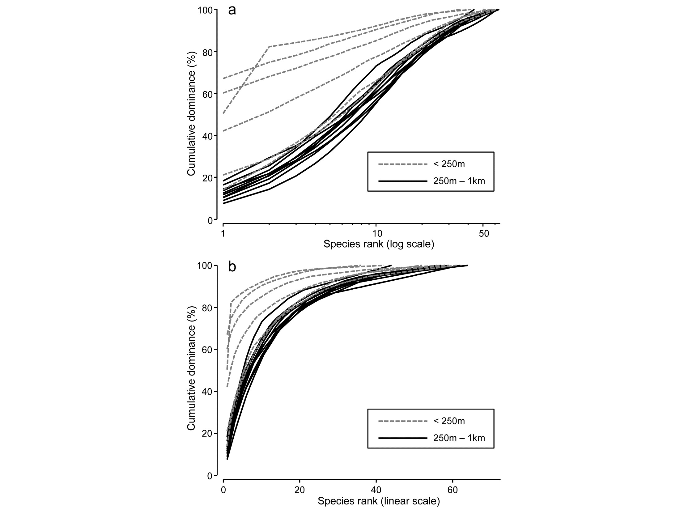
Fig. 8.14. Ekofisk oil-field macrofauna {E}. k-dominance curves for sites in the closest and second closest distance groups to the oil-field, plotted with x axis on: a) log scale, b) linear scale.
For any two curves, in the same or different groups, their absolute distance apart on the y axis, for each x axis point, is calculated and totalled, giving a possible measure of the ‘dissimilarity’ of the two curves. This can be thought of as the area between two curves in Fig.8.14b, taking the value 0 only if they lie totally on top of each other. In Fig. 8.14a, which is the more usual form of a k-dominance curve, the absolute y- axis deviations are given increasingly less weight for larger x-axis ranks, so the distance apart of curves 1 and 2 ($y$ axis values {$y _ {i1}$} and {$y _ {i2}$}) is defined as:
$$ d ^ \prime = \sum _ {i=1} ^ { S _ {\max}} | y _ {i1} - y _ {i2} | \log \left( 1 +i ^ {-1} \right) \tag{8.12} $$
where $S {_{\max}}$ is the largest number of species seen in a single sample and all curves are assumed to continue at 100% after they reach that maximum point. This again effectively defines the ‘dissimilarity’ of two curves in Fig. 8.14a as the area separating them. This is the default for the DOMDIS routine in PRIMER, since this ‘log weighting of species ranks’ matches the standard k-dominance plot, with its emphasis on dominance differences for the most abundant species.
Computing (8.12) among every pair of samples (the output from DOMDIS) and subjecting the resulting dissimilarities to an ANOSIM test of the two distance groups gives R = 0.51 (p<0.3%), a clear difference in dominance structure. The matching test to Fig. 8.14b is little different, with R = 0.56 (p<0.2%).
General curve comparisons: size distributions
The simplicity of a dissimilarity-based approach to testing for significant differences between groups of curves immediately suggests many other contexts in which a similarly robust, multivariate ANOSIM test could be employed. Particle-size distributions in sediment or water-column sampling are often measured in replicate samples, and need comparison between different factor levels in space and/or time. In effect, each curve (whether cumulative frequency or simple frequency polygon¶) needs to be treated as a single, multivariate point, the variables (‘species’) being the differing size classes and their observed values the relative frequencies (i.e. samples are automatically standardised to total to 1 or 100%), or cumulative relative frequencies, and this matrix is input to either Euclidean or Manhattan distance calculation§. The resulting resemblances are then available for the full range of multivariate techniques, including ANOSIM (or PERMANOVA) tests on the groups of replicate curves, ordination by MDS etc.
¶ These are usually not ‘true’ statistical probability distributions, in the sense of individual particles arriving randomly and independently of each other, which would be needed to justify multinomial assumptions for a Kolmogorov-Smirnov test of difference between two such (cumulative) sample distribution functions. Typically, instruments such as Coulter counters will scan vast numbers of particles to construct a size distribution, and the important level of variability is not within a sample but among independent samples taken at the same place or time. Fitting specific parametric distributions, such as a 2- or 3-parameter Weibull, in order to compare parameter estimates among curves, is therefore unappealing: the data is not a true probability distribution and the parametric form will usually not fit well (mixture curves, and even bimodality, may be commonplace), and an unnecessary approximation step is interposed. Comparing simple moment estimators such as mean, standard deviation, skewness (or medians, percentiles etc) of grain sizes in each sample using classic univariate tests is a commonly used and viable alternative, but this may easily miss differences which are due to bimodality or other characteristic shapes repeated across replicates – why not instead just directly compare the curves with each other?
§ PRIMER’s DOMDIS routine is not needed here since this is simply calculation of a distance measure between pairs of samples in a given matrix. DOMDIS’s role in k-dominance curves also includes the initial re-ordering of the matrix in decreasing species abundance order, separately for each sample, before calculating Manhattan distance, in effect, on the resulting matrix. Other distance options given in PRIMER include, for example, the maximum distance of two curves from each other (usually applied to cumulative curves, as in a Kolmogorov-Smirnov statistic). Note that, if no transform is applied to the relative frequency data prior to distance calculation (often the case, though occasionally a mild transform may be preferred, to downweight a dominant size category) then Manhattan distance is equivalent to Bray-Curtis dissimilarity in this case, since the denominator term in equation (2.1) is fixed at 200.