15.6 Examples
Example: Tees Bay macrofauna
Fig. 15.7 shows the nMDS plot for the inter-annual macrofauna samples (282 species) collected every September from 1973 to 1976 in four areas of Tees Bay ({t}, see Fig. 6.17 for map, and individual MDS plots for each area). The current plot uses averages of the 4th-root transformed counts over the four areas (and the two sites within each area), and Bray-Curtis similarities, to obtain an overall picture of the time trend in the benthos. Relating the Bray-Curtis matrix to a triangular matrix of a seriation model, as shown schematically above, the (matrix) Spearman rank correlation ($\rho$) takes a high value of 0.68. Though the stress in the MDS is not negligibly low, the strong time trend seen in this statistic is very evident in the plot. Notice again that is it not at all necessary for the plot to take the form of a straight line to obtain a high $\rho$ value: the statistic is much more general than this and the approximations inherent in any low-d ordination are avoided by direct correlation of the observed and modelled resemblance matrices. High $\rho$ values are triggered by any continuing movement of the community away from its initial state.
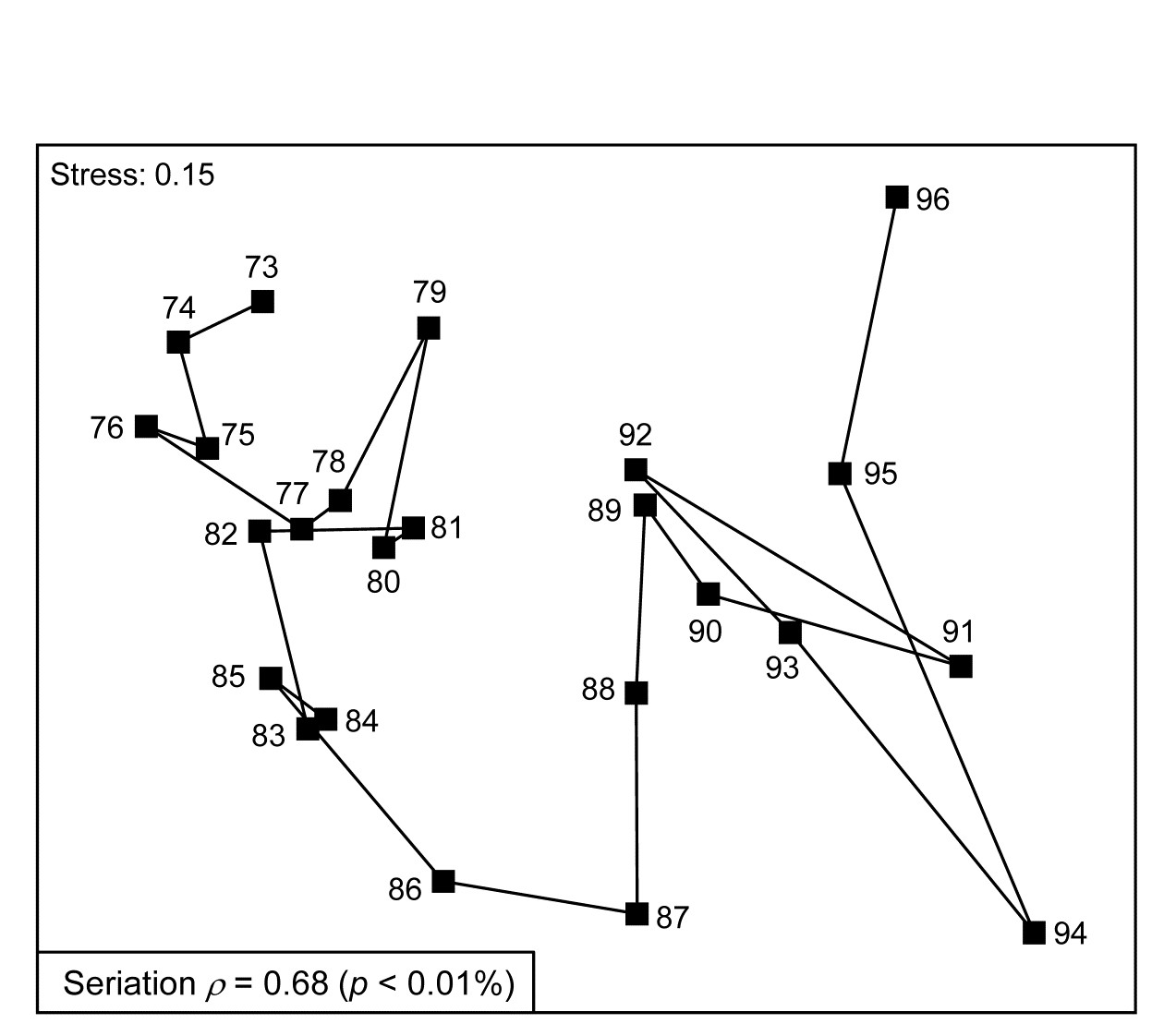
Fig. 15.7. Tees Bay macrofauna {t}. MDS plot of inter-annual time trend in averaged data over 4 areas (and 2 sites per area), for September samples, based on 4th-root transformed counts of 282 species and Bray-Curtis similarities among averaged samples.
As explained above, the hypothesis test available is only of the null hypothesis H$_ 0$: $\rho = 0$, that there is no link of the assemblage to such a serial time sequence, and the null distribution is obtained by recalculating $\rho$ for a large number of random reassignments of the 24 year numbers to the 24 samples. (Note that this is not a test of the hypothesis $\rho = 1$, of a perfect time trend – that is a common misunderstanding!). Here, unsurprisingly, the observed sequence gives a higher $\rho$ than any of 9999 such permutations (p << 0.1%) and is never higher here than about $\rho$ = 0.3 by chance (the large number of years gives a ‘powerful’ test).
The matrix correlation idea can be much more general than seriation, as was seen in Chapter 11, where it was used in the BEST routine to link biotic dissimilarity to a distance calculated from environmental variables. Model matrices can therefore be viewed as just special cases of abiotic data which define an a priori structure, an (alternative) hypothesis which we erect as a plausible model for the biotic data. We wish then to do two things: to test the null hypothesis that there is no link of the data to the hypothesised model, and if rejected, to interpret the size of the correlation $\rho$ of the data to the model.
The model matrix for the Phuket coral data was based on simple physical distance between the 10m-spaced transect positions down the shore. This generalises in an obvious way to the physical distance between all pairs of sampling locations in a geographical layout (indeed this was the distance matrix used by Mantel for his work on clustering of cancer incidences). The test and $\rho$ statistic then quantify how strongly related observed assemblages are to mutual proximity of the samples, and the model matrix can be created by inputting simple x, y co-ordinates (e.g. the decimalised latitude-longitude) to a resemblance calculation of non-normalised Euclidean distance.
Example: Loch Creran/Etive macrofauna
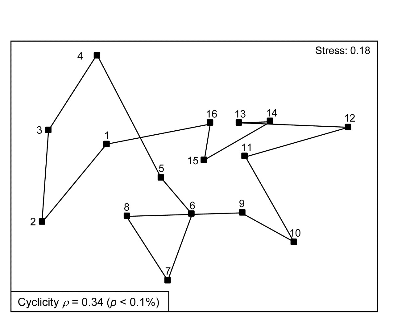
Fig. 15.8. Creran & Etive sea-loch macrofauna {c}. MDS of species abundance data from sub-tidal samples taken at 16 equally-spaced locations on the circumference of a circle (in an unperturbed environment). Significant (albeit weak) match to a cyclic model matrix.
Somerfield & Gage (2000) describe grab sampling of subtidal soft sediments in Scottish sea-lochs, by a vessel positioning at points equidistant (~50m) from a moored buoy, giving 16 equal-spaced samples around a 100m diameter circle (samples numbered 1-16). An MDS ordination from this data set is seen in Fig. 15.8 and while again the stress is high, so the 2-d MDS is not very reliable, there is certainly a suggestion that the samples, joined in their order of sampling, around the circle, match this spatial layout. A model matrix from a serial trend is no longer appropriate of course; instead it will be of the following general form (but illustrated only for 6 points around a circle)¶.
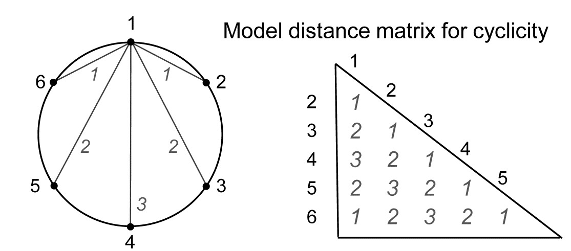
For equal-spaced points round a circle, the inter-point distances shown are not physically accurate – they are chords of a circle, and if that is of radius 1, the actual distances would be 1, 1.73 ($= \sqrt{3}$) and 2, rather than 1, 2 and 3 – but the model matrix is shown with distances 1, 2 and 3 because a Spearman correlation is only a function of the rank orders of the distances.
The matching coefficient of the assemblage (dis)similarities to this distance coefficient is $\rho = 0.34$, and this was larger than produced by any of 999 random permutations of the labels, hence the null hypothesis of no match can be rejected (at p < 0.1%), on a test designed for an alternative hypothesis of cyclicity.
However, rather than a spatial context, a cyclic model matrix is much more likely to be useful in a temporal study, e.g. where seasonality (or perhaps diurnal data) is involved. A data set with monthly levels 1-12, for January to December, would fit poorly to a seriation since the latter would dictate that December was the most dissimilar month to January. An example of bi-monthly sampling, where a test for a hypothesis of no seasonality is not a foregone conclusion, is provided by the Exe estuary nematode data met extensively in Chapters 5 and 11, and also in Chapter 7.
Example: Exe estuary nematodes
Fourth-root transformed nematode counts from 174 species are averaged over the 19 sampling sites of the Exe estuary study {X}, separately for each of the 6 bi-monthly sampling times through a single year. (Note that most previous analyses in this manual have used the data averaged over the months, separately for the sites, though an exception is Fig. 6.12). The question is simply whether there is any overall demonstration of seasonal pattern in these 6 meiofaunal community samples? The model matrix is now exactly that shown immediately to the left and the Spearman correlation of Bray-Curtis dissimilarities with this matrix is 0.21. The evidence in Fig. 15.9 for any such cyclic pattern is unconvincing, either in the MDS or in the formal RELATE test (p = 20%, see inset, where the jagged null distribution is a result of the small number of distinct permutations of the 6 numbers, i.e. 5! = 120).

Fig. 15.9. Exe estuary nematodes {X}. nMDS on Bray-Curtis similarities from counts of 174 species, 4th-root transformed then averaged over the 19 locations, for each of 6 bi-monthly sampling times over one year (1-6). Inset: null distribution for test of cyclicity (r=0.21).
Seriation with replication
Quite commonly, there will be interest in testing for a serial trend in the presence of replicate observations at each of the points in time or space (or at ordered treatment levels etc). This is precisely the problem that was posed towards the end of Chapter 6 (page 6.10 onwards) in setting up the ordered ANOSIM tests. There are now ordered groups of samples (A, B, C, …), and the null hypothesis ‘H$_ 0$: A=B=C=…’ that the groups are indistinguishable is not tested against a non-specific alternative ‘H$_ 1$: A, B, C, … differ’ but against the ordered seriation model ‘H$_ 1$: A<B< C …’. More detail is given on page 6.10 to page 6.12 , but the only difference here is that instead of using the generalised ANOSIM statistic $R ^ 0$, the slope of the regression line of the ranks {$r _ i$} in the (biotic) dissimilarity matrix against the ranks {$s _ i$} in the model matrix, we use here their correlation $\rho$ (this is Pearson correlation on the ranks, i.e. Spearman on the matrices).

The simple form of seriation with replication (the model matrix for which is seen above, illustratively, for 3 groups A, B, C, with 2 replicates in groups A and C, and 3 replicates in B), was extensively studied by
Somerfield, Clarke & Olsgard (2002)
and illustrated by further Norwegian oilfield benthic data from the N Sea, {g}.
Example: Gullfaks oilfield macrofauna
Routine monitoring of soft-sediment macrobenthos around all the Norwegian oilfields typically involves sites radiating in several directions (usually 4) from the centre of each field (as in the Ekofisk study, see Fig. 10.6), but for analysis purposes broadly grouped into distance classes. For the two oilfields: GullfaksA (16 sites, 1989 data) and GullfaksB (12 sites, 1993), 3 groups were defined as C: <1km, B: ~1km, A: > 1km from the centre of drilling activity, each consisting of between 4 and 6 replicate sites. These are shown as differing symbols and shading on their faunal MDS plots in Fig. 15.10. Unlike the Ekofisk data, where the oilfield had been operating for longer, the group differences are less clear-cut, and differences are not significantly established in unordered ANOSIM tests.
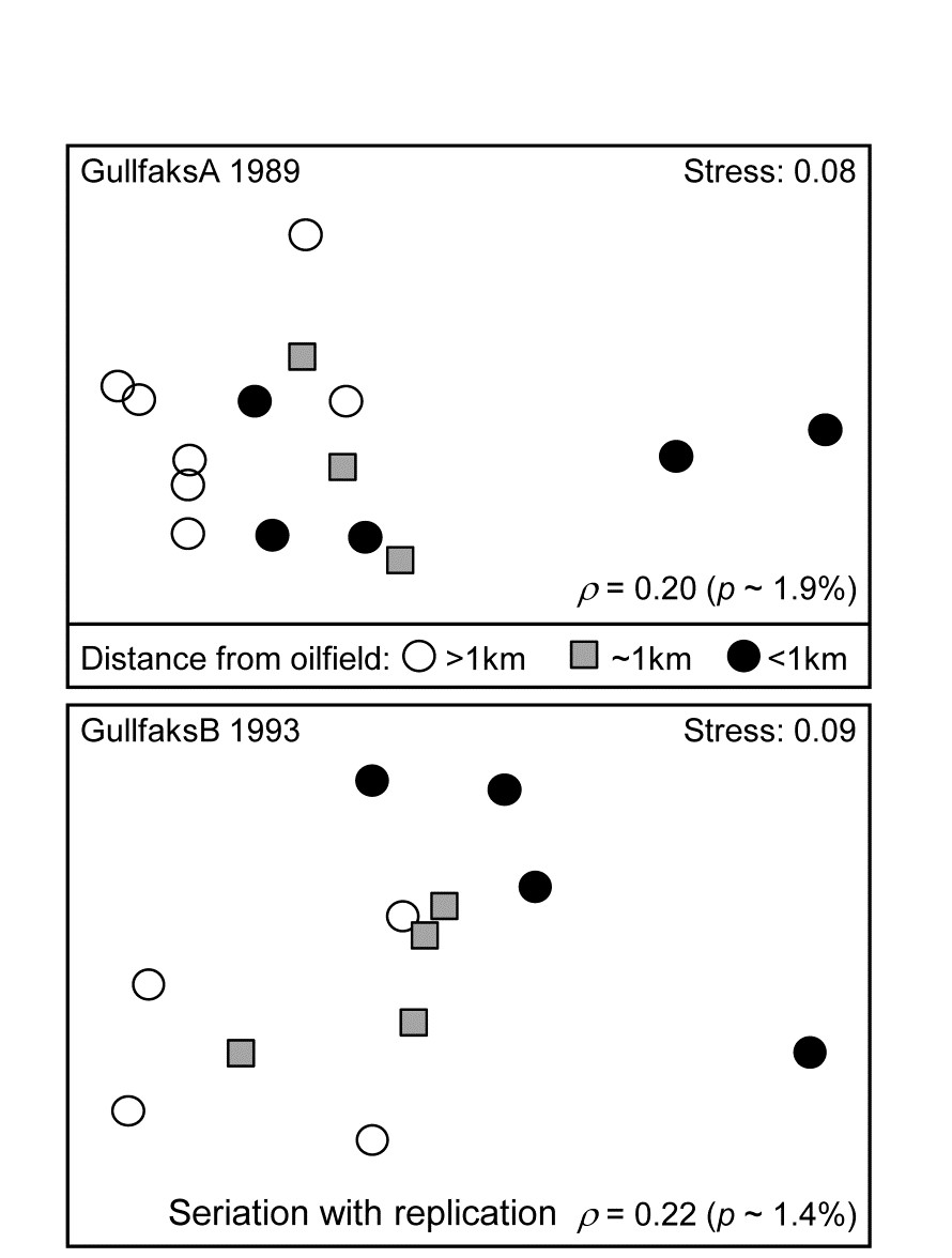
Fig. 15.10. Gullfaks oilfields, macrofauna {g}. nMDS on Bray-Curtis similarities from transformed species counts for sites in 3 distance groups A: >1km, B: ~1km, C: <1km from the oilfield centres. Both show a significant left to right progression, with seriation statistics $\rho$ =0.20 and $\rho$ =0.22 for GullfaksA and GullfaksB fields respectively.
However, when tested against the ordered alternative, using the seriation with replication schematic (above) the $\rho$ values of 0.20 and 0.22 are both significant at about the p < 2% level. The issue here is one of power of the test. As Somerfield, Clarke & Olsgard (2002) show, where a test against an ordered alternative is relevant, it will have more power to reject the null hypothesis (‘no group differences’) in favour of that alternative†. The improved power always comes at a price though, namely the likely inability to detect an alternative which is not the postulated model matrix. Thus, in Fig. 15.10, B is generally intermediate between A and C, and this is as postulated. If the benthic community is distinct at differing distances from the oilfield as a result of dilution of contaminants coming from the centre§, then a situation in which groups A and C have indistinguishable benthic assemblages but B has a different one would not be interpretable, and would be discounted as a ‘fluke’. If we are happy to forgo the prospect of ever detecting such a case then it makes sense to focus the statistic on alternatives that are of interest, and thereby gain power.
Constrained (‘2-way’) RELATE tests
Just as was seen with the BEST procedure in Chapter 11 (page 11.5), it is straightforward to remove the effect of a further (crossed) factor when testing similarities against a model matrix (or any secondary matrix). The $\rho$ statistic is calculated separately within each level of the ‘nuisance’ factor, so that any effect of the latter is removed, and the resulting $\rho$ statistics then averaged. The same procedure is carried out for the permutations under the null hypothesis, i.e. it is a constrained permutation in which labels are only permuted within the levels of the second (nuisance) factor, just as in 2-way ANOSIM or its ordered form (page 6.5 and page 6.12). However, the ordered ANOSIM tests in PRIMER v7 only implement the seriation model (with or without replication), so the following RELATE example illustrates a 2-factor case where a cyclic test is needed on (replicated) seasons, having removed regional differences in the assemblages, {l}.
Example: Leschenault estuarine fish
Veale, Tweedley, Clarke et al. (2014) describe nearshore trawls for fish abundance (43 species) in a microtidal W Australian estuary, with freshwater inflow only near the estuary mouth (Basal region, B) and thus a reverse salinity gradient increasing through its Lower (L), Upper (U) and Apex (A) regions. That region has a strong effect on fish communities is evident from the MDS of Fig. 15.11b, for 6-8 replicate samples (both spatially, in regions, and temporally, across years) from each of 16 combinations of 4 seasons and 4 regions. There is some suggestion from Fig. 15.11a (the same MDS but showing seasons) of a seasonal effect, but this is hard to discern, given also the strong regional effect.
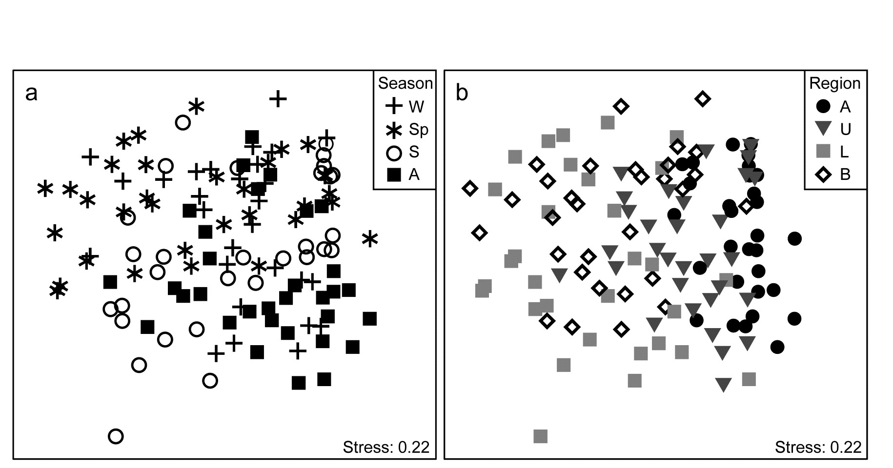
Fig. 15.11. Leschenault estuary fish {l}. nMDS from Bray-Curtis on dispersion weighted then $\sqrt{}$-transformed samples of counts from 43 species, of sites within the four regions (Apex, Upper, Lower, Basal) over two years and in all seasons of each year (Winter, Spring, Summer and Autumn). a) and b) are the same MDS but indicate samples from seasons & regions respectively.
The conditional test for seasonality fits the model matrix on page 15.6, but for only 4 not 6 times (Autumn, Winter, Spring, Summer) and with replication. (A test without replication is possible but this really needs to be for monthly or bimonthly data rather than just four seasons, since there are only 3! = 6 distinct permutations from a single set of 4 times). The $\overline{\rho}$ statistic, averaging the cyclicity (seasonality) $\rho$ values, given by each region separately, is only 0.27, indicating the high replicate variability (seen in Fig. 15.11a and b), but this is strongly significantly different from zero (p<<0.01%) since the permutations never came close to producing an average $\rho$ larger than 0.1. That there is a clear seasonal effect, consistently across regions, can be seen (as must always be done, and rarely is!) by averaging over the temporal and spatial replicates to obtain the 16-sample nMDS of Fig. 15.12.
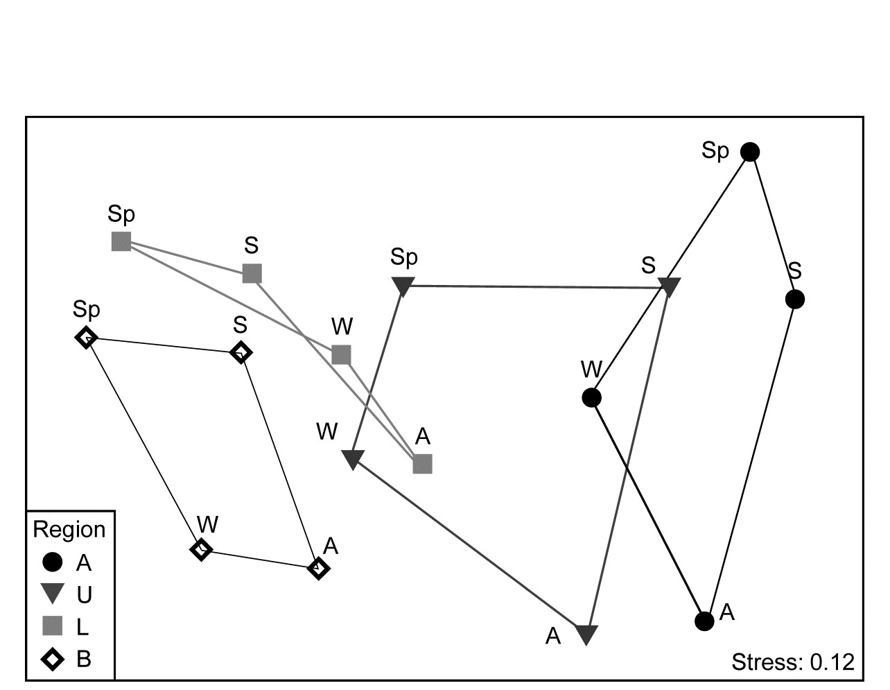
Fig. 15.12. Leschenault estuary fish {l}. nMDS from Bray-Curtis for averages over all samples (previously dispersion weighted then transformed, page 9.6) from 4 regions over 4 seasons. Regions align left to right in increasing salinity up the estuary, clearly with parallel seasonal cycles.
¶ The PRIMER RELATE routine gives three options: match to a simple seriation (distance matrix of the type on page 15.5), simple cyclicity (distance matrix as seen here) or to any other supplied triangular matrix (a further model matrix, or possibly a second biotic resemblance matrix, e.g. testing and quantifying the match of reef fish community structure to the coral reef assemblages on which they are found). A separate routine on the Tools menu, Model Matrix, allows the user to create more complex models, for seriation or cyclicity where spacing is unequal or where there are replicates at each point. These are specified by numeric levels of a factor. E.g. though this simple 6-point circular model is automatically catered for by RELATE, recreating it using the Model Matrix routine needs a factor with levels in (0,1), taken to be the same point at the start and end of the circle, i.e. use levels 0, 0.167, 0.333, 0.5, 0.667, 0.833 for the samples 1, 2, 3, 4, 5, 6.
† This is certainly true of the analogue in univariate statistics (see Somerfield, Clarke & Olsgard (2002) ), e.g. the choice between ANOVA and linear regression when treatment levels (with replication) are numeric. Regression is always the more powerful, though it would completely miss, for example, a hormesis response that ANOVA would detect. Power is a much more difficult concept in multivariate space but Somerfield, Clarke & Olsgard (2002) demonstrate a similar result for unordered ANOSIM vs RELATE (i.e. ordered ANOSIM) in some special cases, by simulation from observed alternatives to the null of ‘no change’.
§ Or a number of other causal mechanisms to do with existence of the oilfield that might be tricky to distinguish by biotic observational data alone, e.g. a change in the sediment structure resulting from deposition of finer grained drilling muds, maybe disruption of current flows, even reduced commercial fishing pressure etc.