7.3 Example: Amoco-Cadiz oil spill
A second example of deriving sets of coherent species curves, this time temporal rather than spatial, is for the benthic macrofauna sampled at one site in the Bay of Morlaix, on 21 occasions over 5 years, spanning the period of the Amoco-Cadiz oil tanker spill, for which the samples MDS and clustering were in Fig. 5.8, {A}. This is a more challenging example because many of the same species are present throughout the period, so Type 3 SIMPROF groups will not identify subsets of species which are exclusively found only in different groups of samples. In fact, Type 2 SIMPROF (see the plot in Somerfield & Clarke (2013) gives very little, if any, evidence of an excess of negative associations: species do not appear to be ‘excluding’ other species (by competitive interactions or by independent but opposite responses to seasonal or other environmental changes), on any substantial scale at least. Again 52 species, coincidentally, were retained from the large original set of 251, these being all the species which accounted for at least 0.5% of the total abundance at one or more of the 21 sampling times.
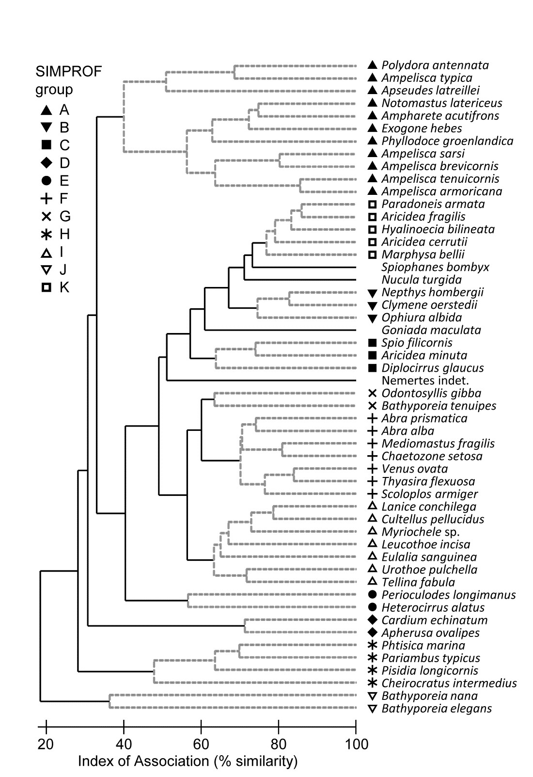
Fig. 7.5. Amoco-Cadiz oil spill {A}. Dendrogram (agglomerative, group average linked) from an index of association matrix among 52 macrofaunal species, each of which accounts for at least 0.5% of the total abundance at one or more of the 21 sampling times. Grey dashed lines and differing symbols denote the 11 ‘coherent groups’ (A-K) containing more than one species, from 5% level Type 3 SIMPROF tests. There are a further four singleton groups, similar to B, C and K, not displayed in the subsequent line plots.
Fig 7.5 shows the species cluster analysis, based on the index of association computed on untransformed species counts, standardised to total 100 over the times. Type 3 SIMPROF tests yield 15 distinct species groups (A-K), and standardised counts for 11 of them appear as component line plots in Fig. 7.6. These demonstrate a wealth of fascinating biological information on the coherent responses of groups of species, seasonally and in response to the oil spill year and potential recovery over the next three years. The groups are arranged in approximate order A-J of a move of peak abundance towards the later times, with species in K showing consistent abundances (they are always present) and little convincing evidence of temporal patterns at all. The large A group, which contains a number of Ampelisca species found in high densities prior to the oil spill is characterised by virtual non-recruitment in the spill year and then a gradual recovery of its seasonal cycle, though not generally to the same peaks by the 5th year. Group B has something of the same pattern though with an apparently fuller recovery. Groups D and E appear to show an opportunist response to the spill, with peak numbers in the year immediately following, whereas F species are of consistently low abundance pre-spill but this starts to rise a year or so later, peak and then fall away in the 5th year; it is a group without a very clear seasonal pattern. Group I has a similar structure but the rise is more delayed still, and the seasonal pattern perhaps more evident; the latter is more marked still in H, and so on. Of course, some of these temporal patterns may simply be the result of natural inter-annual variability driven by a range of environmental factors and, without a spatio-temporal control/reference structure, inference about the causes for any particular patterns has to be suitably guarded. But what is unarguable is that the Type 3 SIMPROF technique has pulled out an apparently convincing set of differing temporal responses – consistent within a group, distinguishable between groups – a combination of patterns which is synthesised in the multivariate pattern of the nMDS, with its obvious change, partial recovery and re-establishment of the seasonal cycles.
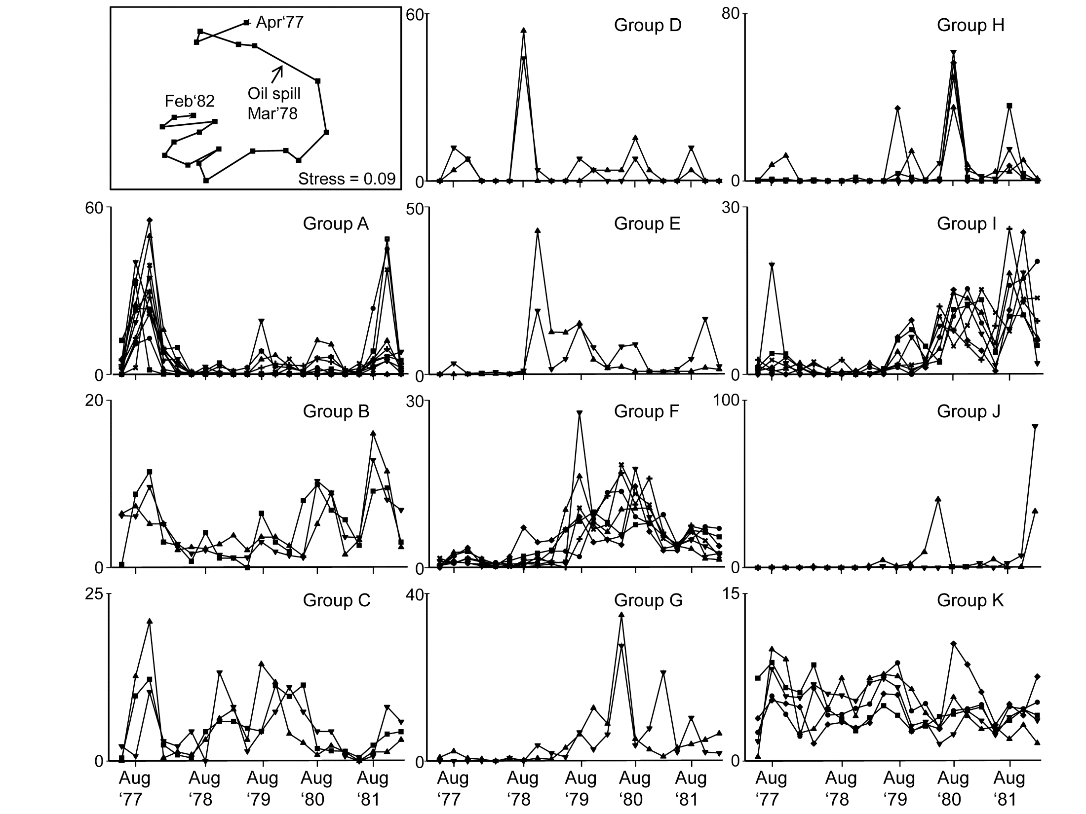
Fig. 7.6. Amoco-Cadiz oil spill {A}. 'Coherent species curves’ for the SIMPROF groups A-K of Fig. 7.5. Also re-shown (top left) is the nMDS plot Fig. 5.8a of the 21 samples over 5 years, displaying community change and partial recovery, with the seasonal cycle re-established. Note that this MDS is based on heavily transformed (4th root) abundances so its similarities do draw from a wide range of these species patterns. The explanation of the clear MDS structure is seen in the combination of differing responses from the various species sets.
Some general points about Type 3 SIMPROF tests
-
As pointed out on the footnote on page 7.2, a Type 3 test is impossible to perform with only two species, so where a group of two is split from other clusters, as for the two Bathyporeia species, group J above, it cannot be further subdivided, whatever the association is between the species. Nonetheless, it will be distinct from other groups and (as here) the two species must have some common association otherwise they will be sliced off from the larger cluster as singletons. Naturally this raises the issue of the power of the SIMPROF test and much the same comments apply as for Type 1 tests, see the discussion on page 3.5 (though you will need to mentally transpose ‘samples’ and ‘species’!). In brief, though power to further divide a group is difficult to define formally in a multivariate context, it will clearly increase with the number of species in the group and especially with the number of samples over which the association is calculated. Thus, a time series of just 4 seasons will tend to lead to fewer and larger species groups than for a series of 12, monthly, samples. Large spatial or long temporal series could distinguish fine-scale, and somewhat trivially different, sets of species responses. Judicious use of averaging (but not over-averaging) may be needed if there is much ‘noise’ in the data, so that more genuine ‘signals’ are compared.
-
It is worth re-iterating the point that Type 3 tests require an association measure with an inbuilt species standardisation (such as equation 7.1) and entry of a matrix which has already been standardised. Tempting though it is to feel that: a) input of an unstandardised matrix and use of the index of association; or b) input of a standardised matrix and use of the normal Bray-Curtis measure (applied to the species, equation 2.9) will both do the trick, this is wrong – both will give results which are incorrect. The first is more plainly wrong, as noted in the footnote on page 7.2 but the second will, more subtly, make the test unconservative, leading to a greater number of smaller-sized groups. Whilst the real similarity profile will be fine, since the index of association is just Bray-Curtis on standardised data, after the permutations the species are no longer exactly standardised, so the permuted profiles will tend to contain (artefactually) lower similarities, making the real profile’s larger values appear more significant.
-
Whilst the Exe estuary and Morlaix examples above both appeared to work well with standardising a data matrix which had not been previously transformed, it is not clear that this is always the best approach. Species standardisation removes the sometimes very large disparity between abundances of different species (e.g. between large and very small-bodied organisms) but it does not address erratically large counts across samples for the same species. Pre-treatment by transformation is sometimes needed to tackle these outliers, as well as to better balance contributions from abundant and less abundant species, in which case it would make perfect sense to transform prior to standardising ‘noisy’ data, before input to Type 3 tests. It is perhaps not entirely coincidental that the Exe and Morlaix data matrices were both averaged (over seasons and over replicates), reducing the severity of any such outliers.
-
Though this chapter concerns only species variables, it is clear that Type 3 SIMPROF tests are much more widely applicable, to other measures of association or correlation and to environmental variables or biotic variables which are not positive (or zero) ‘quantities’, as in an abundance matrix. Somerfield & Clarke (2013) give examples of Type 3 tests for both classes of variables: an environmental suite of heavy metals and organics in the Garroch Head study {G}, and a biomarker study of biochemical/histological ‘health’ indices from flounder sampled along a North Sea transect (see the PRIMER User manual for the data source). Standard Pearson correlations are relevant as association measures in both cases, sometimes with (differing) transformation of individual variables. The only new issue that arises is that, for the biomarker data at least, whether correlations between variables are positive or negative is not of primary concern – some biomarkers increase when an organism is subject to anthropogenic impact and some decrease. This is best handled by reversing some variables so that all are expected to decrease (say) under impact, so that the range of associations go from ‘uncorrelated’ to ‘exactly correlated’ variables – there is no longer a meaningful concept of ‘strongly negatively correlated’. In precise analogy with the species examples, matrices need to be normalised (after any transformation) before entry to Type 3 tests using Pearson correlation, and ranked before tests using a Spearman rank correlation.
In conclusion
Ultimately, like most of the techniques in PRIMER, coherent species curves are fundamentally simple and transparent. Indeed, practitioners have been drawing line plots of species responses over spatio-temporal gradients throughout the history of ecology, but they have usually been for single species or combinations that are arbitrarily selected. What Type 3 SIMPROF tests do is to give some objectivity to the selection of species to place in the same component line plot and provide a statistical basis for inferring differences in pattern between, and similarity within, components.