1-way ordered ANOSIM (Ekofisk oil-field study)
However, for the Ekofisk oil-field study of the last section there is a postulated cause for benthic community change (the presence of an oilfield) and impacts, if any, are expected to result in a monotonic change with increasing distance from the drilling centre. For the four distance groups, defined prior to the data analysis: D (<250m), C (250-1000m), B (1 - 3.5 km) and A (>3.5km), a test of the null hypothesis H$_0$:A=B=C=D against the ordered alternative H$_1$:A$\rightarrow$B$\rightarrow$C$\rightarrow$D (or vice-versa) is entirely appropriate, and inability to detect the above scenario (sites near and far from the rig being similar but intermediate sites differing) would usually be a price well worth paying in pursuit of a more powerful test of this specific (ordered) alternative hypothesis. [We return to this point, and example, in Section 14, based on the seriation with replication test of Somerfield PJ, Clarke KR & Olsgard F 2002, J Anim Ecol 71:581-593, which tackles the same problem with a slightly different (RELATE) statistic, $\rho$. The relationship of the new, ordered ANOSIM statistic to that for the previous Analyse>RELATE test is covered in Chapter 6 of CiMC].
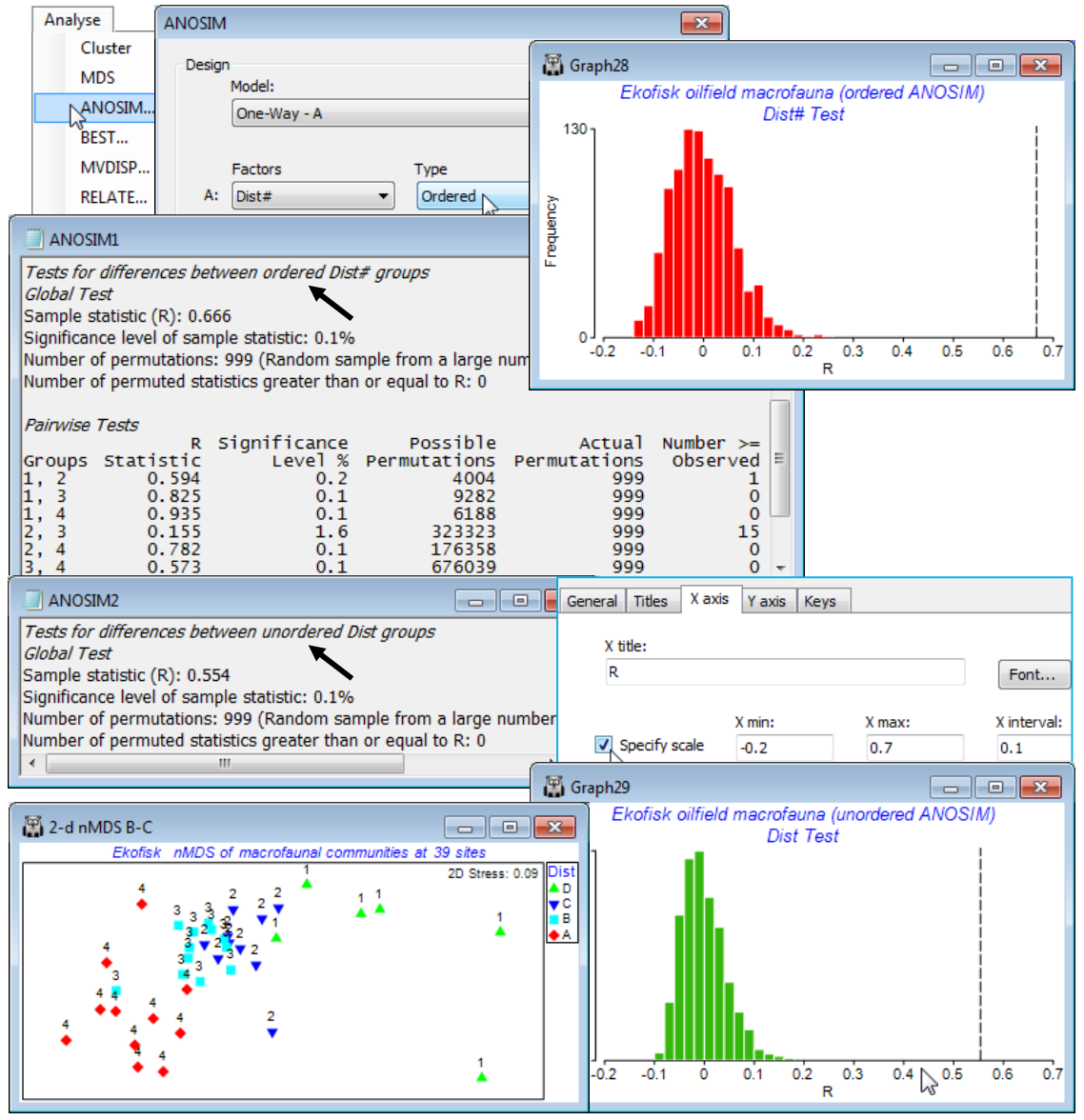
Re-open the Ekofisk ws workspace of Section 8, in which the data Ekofisk macrofauna counts from C:\Examples v7\Ekofisk macrofauna has been square-rooted and input to Bray-Curtis calculation, giving resemblance matrix B-C on sq rt. On this, take Analyse>ANOSIM>(Model•One-Way-A)> (Factors A: Dist#)>(Type Ordered). Note that the numeric form Dist# (levels 1-4) of the factor representing distances from the oilfield is required for the Ordered ANOSIM test; the alphabetic form ins>Dist (levels D-A) is not recognised by PRIMER as an ordering (if Dist# is not available, re-create it by Edit>Factors>Add>(Add factor named: Dist#), and enter 1 at the top, opposite the first D, 2 opposite the first C, 3 when it changes to B, and 4 to A, then highlight the column and Fill>Value to fill in all the blanks appropriately).
The outcome is an ordered R$^\text{O}$ of 0.67 which, as can be seen from the null distribution histogram, unquestionably rejects the null hypothesis (R$^\text{O}$ = 0) on a p<0.1% level test (i.e. P<0.001), and would do so for massively smaller values of p. The ensuing pairwise tests show a clear pattern of increasing R for increasing separation of the distance groups, exactly as one would expect from a serial community change. Only the differences between groups 2 and 3 (C and B) are at all border-line, with a low R of 0.16 (but still significant in conventional terms, at the 2% level). Note that the pairwise tests are always ordinary R statistics – there is no difference between an ordered and an unordered test when there are only two groups! Now re-run the ANOSIM specifying the unordered case, this time using either the alphabetic or numeric factors Dist or Dist# (it no longer matters). The R = 0.55 value, though still massively significant, is seen to be lower than the R$^\text{O}$ = 0.67 of the ordered test. These statistics are directly comparable, and show the better fit of the underlying model (see Chapter 6, CiMC) of equi-stepped serial change than that of equi-different groups. This is clearly evident also from the previous nMDS plot. Save and close the workspace Ekofisk ws.

