Metric MDS; (Great-circle distances for world cities)

A significant new feature in PRIMER 7 is the construction of metric MDS ordinations (mMDS), together with variations such as threshold mMDS (tmMDS) and a specific combination of nMDS and mMDS; the rationale and details are fully covered towards the end of Chapter 5 in CiMC. The mMDS algorithm operates in a very similar way to nMDS, by an iterative search for an optimal configuration of samples in a specified dimension (or, in practice, a range of dimensions). The key difference is in the Shepard diagram, which is constrained to be fitted by a straight line through the origin (i.e. two points should only be represented as coincident if their dissimilarity is 0), as a result of which mMDS has axis measurement scales. Under conditions of low stress and a well-fitting line in the Shepard diagram, the distances in the plot are thus directly interpretable as the dissimilarities/ distances in the original resemblance matrix. This is only likely to happen, however, either for a resemblance matrix that is close to behaving like Euclidean distances in the first place, e.g. from an environmental analysis using normalised Euclidean distance, or where there are only a handful of samples to ordinate, e.g. for some means plots. In such cases, mMDS has significant advantages over nMDS; in normal community analyses nMDS will usually be much superior.

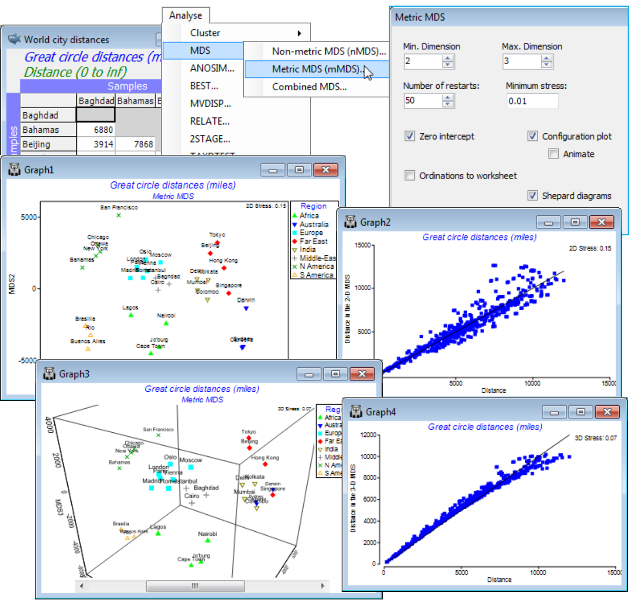
A data set for which the resemblance matrix appears unequivocally suited for mMDS is discussed in CiMC Chapter 5 and given in directory C:\Examples v7\World cities, data World city distances. This is a physical distance matrix in the first place, being a triangular matrix of the (great-circle) distances round the globe between all pairs of 33 world cities (drawn from The Reader’s Digest Great World Atlas, 1962). Run Analyse>MDS>Metric MDS (mMDS) under the defaults, to give both a 2-d and 3-d map of these (3-d) cities, along with their associated Shepard diagrams.

You will probably need to Graph>Flip X or Y and Rotate Data to get the standard 2-d orientation of world maps, and also Rotate Axes for the 3-d plot, though the arbitrariness of compass points (N at the top etc) is clear! Note how the axis scaling on the mMDS plot subtly changes as the data is rotated within the plot, as it needs to do in fully preserving the meaning of distance. Though the 3-d mMDS does place the cities in roughly the correct relation to each on the surface of a sphere, it may initially be a surprise to see that this 3-d picture of 3-d distances has non-negligible stress (of 0.07). The clue is in the Shepard diagram, which shows that the data is trying to force the relation away from the fitted straight line of the metric solution towards a curve, especially for the larger distances. Remembering that the matrix is of great-circle distances (direct air miles) but the 3-d MDS represents through the Earth distances resolves the issue. The true relationship is not linear and, even for this (apparently simple) physical distance matrix, nMDS is superior, placing the cities perfectly correctly on the globe surface, with stress 0, and marginally reducing the 2-d stress.