(Ekofisk oilfield macrofauna)

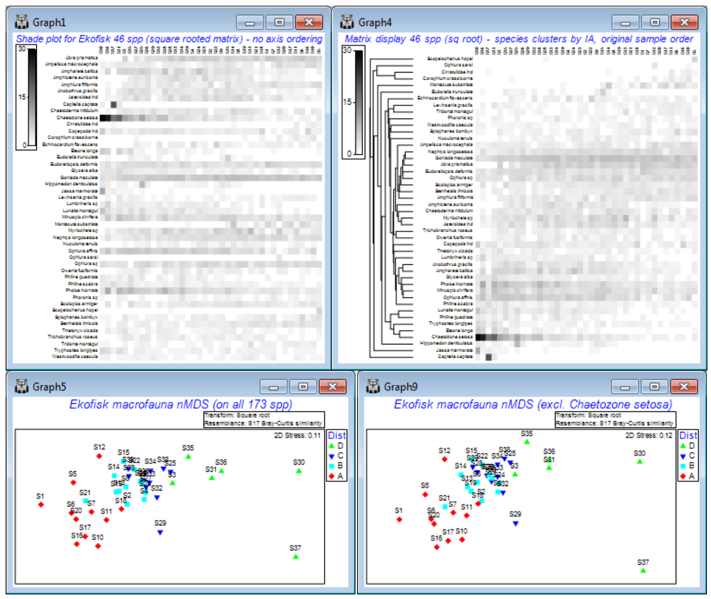
A good example of how ordering of species in a shade plot can aid interpretation is seen for macro-benthic communities at different distances from the Ekofisk oilfield, last saved in Section 9 but which we have seen several times since it was introduced as the first example data set, in Section 1. These data have been run through Plots>Shade Plot before, in the discussion of transformation options in Section 4, where it was clear that unless some sort of transform was applied (square root looked the best bet), the effect of a single species (Chaetozone setosa) would dominate the result of a multivariate analysis. We remarked at the time that it was not immediately clear from the shade plot that, even after transformation, there would be a convincing relationship between the species communities and the distance from the oilfield of each of the 39 samples (note that the sample order in the matrix is of increasing distance from the oilfield, across the columns from left to right, and the species order in the rows is alphabetic, and this order will be unchanged by a simple run of Plots>Shade Plot). Yet we have since seen (in Section 8) a highly convincing nMDS plot of the gradient of change in community structure (on root transformed data and Bray-Curtis similarities) with distance to the oilfield, backed up by a strong 1-way ordered ANOSIM test result in Section 9. It might be argued from the shade plot shown earlier, and repeated below (left), that for the mild square-root transform, Chaetozone setosa will still have rather a strong input to this analysis – and it certainly has increasing values as sites gets closer to the oilfield. But the nMDS is repeated below after omitting this species and the convincing gradient pattern is little changed. Why this is so does become clearer, however, when we run the original data matrix through Matrix display, and re-instate the original sample order on the x axis – because of the clustering/seriation on the species axis we can now see groups of species which are: a) mainly restricted to the ends of the gradient; b) steadily increasing or decreasing with distance from the oilfield; c) in between those – species that increase then decrease along the gradient. It is a combination of all of these that gives a clear MDS.

So, to avoid cluttering the existing Ekofisk ws for later (Section 14), open into a clear workspace Ekofisk macrofauna counts from C:\Examples v7\Ekofisk macrofauna and take Select>Variables> (•Use those that contribute at least 2 %) which retains 46 species, and Pre-treatment>Transform (overall)>(Transformation: Square root). On the result, run Plots>Shade Plot to obtain the left-hand plot below (as in Section 4). In contrast, Select>All on Ekofisk macrofauna counts, and take Wizards>Matrix display>(✓Reduce species set>Keep most important: 46) & (Transformation: Square root) and uncheck (✓Retain sample groups). The same 46 species are retained, as are the matrix entries, but species are re-ordered. So are the samples, which have now been clustered and seriated (subject to the constraints of their dendrogram) on the x axis, but this needs to be removed with Graph>Special>Reorder>Samples>(Order•Original) & (Constraint•None), whilst leaving the Variables side of this dialog unchanged. The only other change is to set (No. of seriate restarts: 999 or 9999). OK takes you back to the initial Special dialog – note that although (✓Draw sample constraint group boundaries) is ticked, no lines divide up the shade plot because (Constraint•Factor groups       ) was not specified on the Reorder dialog. The shade plot to the right, below, is the result. Under the shade plots are the nMDS ordinations, left: from all 173 species of Ekofisk macrofauna counts (root-transformed, then Bray-Curtis); and right: having omitted Chaetozone setosa by Edit> Clear Highlight, highlighting just that species, Edit>Invert Highlight and Select>Highlighted, then running root-transforms, Bray-Curtis similarities and nMDS in just the same way.

The interesting point about the re-ordered shade plot (right), which is worth re-iterating, is that the row and column orderings are independently derived. Looked at from the point of view of species rather than samples, the species index of association (IA) matrix is used to place species in their natural order, in terms of the differing similarities of their counts over samples, but it would be identical for any re-ordering of the samples. The sample ordering is fixed by an external factor – distance to the oilfield centre. Hence, if you can discern any diagonalisation of the matrix in this plot then that must be evidence for a serial relation of the community composition to distance from the oilfield. And that is what is now observed, and is picked up by the MDS and ordered ANOSIM. But, equally clearly, it is a subtle, whole community property that is being captured.

Close the workspace – save as Ekofisk ws2 if you wish, but we shall only need Ekofisk ws later.