3-way crossed ANOSIM (King Wrasse diets)

A dietary study of W Australian fish concerns composition by the volume of taxa (21 broad dietary categories: gastropods, bivalves, annelids, etc) in the foregut of King Wrasse from one of 4 length-classes, caught in 3 locations in 2 periods of the year and 2 replicate times of sampling within each period (each replicate is a similar-sized pool of gut content of fish in each length-class). The data is Wrasse gut composition in C:\Examples v7\Wrasse diets. More detail is given in Chapter 6, CiMC; the analysis is from a wider study by Lek E et al 2011, J Fish Biol 78: 1913-1943.

This is an example of a 3-way fully crossed design with replication, ABC, with A: location, B: length and C: period. A test of the null hypothesis of no effect, of each of the factors in turn, simply uses the earlier 2-way crossed design, e.g. with first factor A and second the flattened BC factor. The latter places all combinations of the levels of B and C in a single factor (using Edit>Factors>Combine and placing the B and C factor names in the Include box). The 2-way test for factor A now therefore constructs a 1-way ANOSIM R statistic for each combination of levels of B and C, and averages those, testing this against permutations constrained to stay within the B$\times$C levels. The same procedure is followed for each factor, so B is tested having removed the effect of A$\times$C, and C is tested have removed any effect of both A and B (or their interaction). So, whilst this could all be carried out by three separate runs of 2-way crossed ANOSIM, it is more conveniently (in PRIMER 7) performed by specifying the 3-way crossed design A$\times$B$\times$C. The resulting three average R values can then validly be compared, to determine the relative overall magnitude of the three effects.

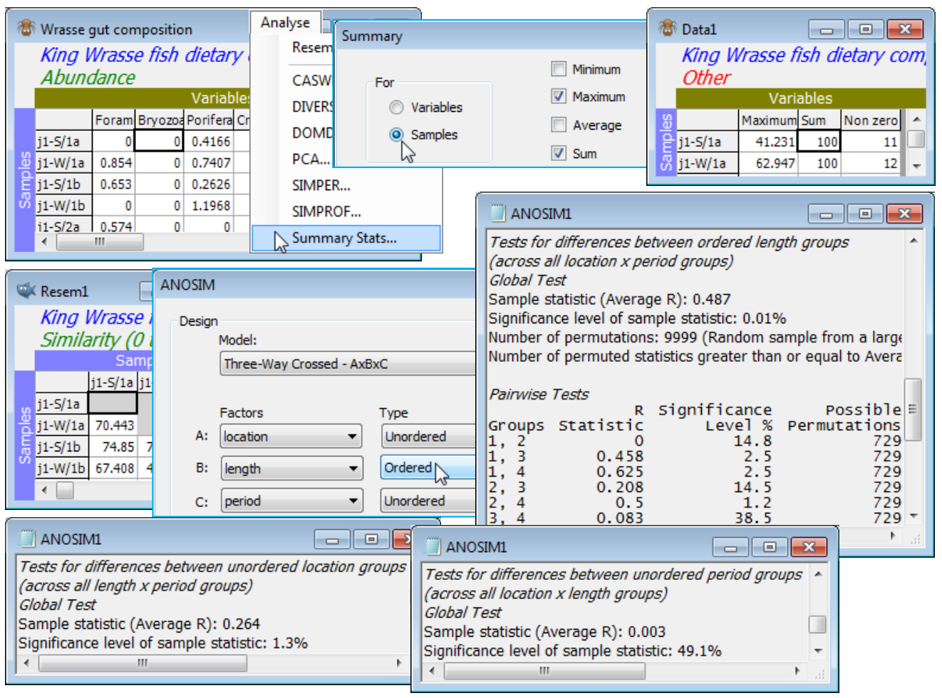
Here, the 3 levels of the location factor are not ordered, and there are only 2 periods (so whether treated as ordered or not is immaterial), but the 4 length classes of the predator wrasse are clearly ordered – the expectation is that, if the diet changes at all, it will do so in progressive fashion as the fish matures. So, check that the samples are already standardised to add to 100% across the dietary categories by Analyse>Summary Stats>(For•Samples) & (✓Sum) – you may want to leave other boxes checked also – and square-root transform then compute Bray-Curtis similarities, and input to Analyse>ANOSIM>(Model: Three-Way Crossed - AxBxC)>(Factors A: location) & (B: length) & (C: period), with B Ordered, specifying (Max permutations: 9999). The average R values show that B (0.49, p<0.01%) is the largest effect, then A (0.26, p<1.5%), but that C has no effect at all (0.00). The pairwise average R values for the length-class effect show the increasing differences in diet with difference in fish lengths, exactly as would be expected for an ordered factor (you may wish to re-run the analysis for an unordered B factor and note how this reduces its global average R value).

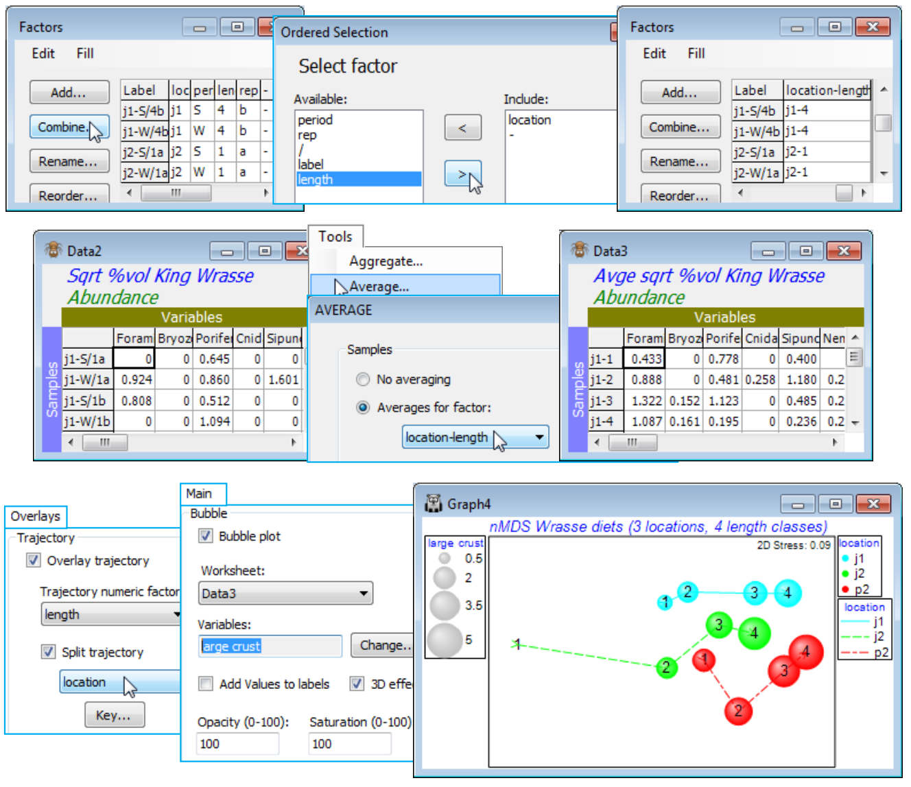
Given the clear absence of a period effect, a useful summary would be to average the (transformed) data over both the replicates and the periods (by Tools>Average and supply the combined factor for AB), recalculate the similarities and enter nMDS. The plot exemplifies a split trajectory, with Special>Overlays for length, splitting by location; you might also like to recreate the bubble plot of Fig. 6.15 of CiMC by adding a dietary component. Save and close the workspace (Wrasse ws).