(Sea-loch contiguous macrofauna cores); Species accumulation plots

The final set of data in this section is of a benthic study by Gage JD & Coghill GG 1977, in Coull B (ed) Ecology of marine benthos, Univ S Carolina Press, at a single site (C-12) in Loch Creran, Scotland, involving 256 contiguous cores arranged along a single transect. Small cores were used to examine local-scale dispersion (clumping) properties of sediment macrofauna. The data matrix of 67 species by 256 samples is the file Creran macrofauna counts in directory C:\Examples v7\ Sea-loch macrofauna; open this into a new workspace. It will be used here to illustrate the final type of curvilinear plots available in PRIMER, species accumulation curves.

The Plots>Species Accum Plot routine plots (and lists) the increasing total number of different species observed (S), as samples are successively pooled (often referred to as the S obs curve). This is accessed when the active sheet is any species $\times$ samples matrix (though for all except the Chao1 index, see later, which requires genuine counts, only the presence/absence structure is used). There are three options for the order in which samples in the data sheet are successively amalgamated: (Sample order•Original), (•User defined) or (•Permute). The first case simply takes samples in their label order in the worksheet and the second specifies the order by a Select samples button. This provides an Ordered Selection dialog, in which samples can be moved up or down with the usual buttons – alternatively, re-order the original sample labels with Edit>Sort, using a factor. The third (default) option is to enter samples in random order, this being carried out 999 times (or whatever specified) and the resulting curves averaged, giving a smoothed S curve.

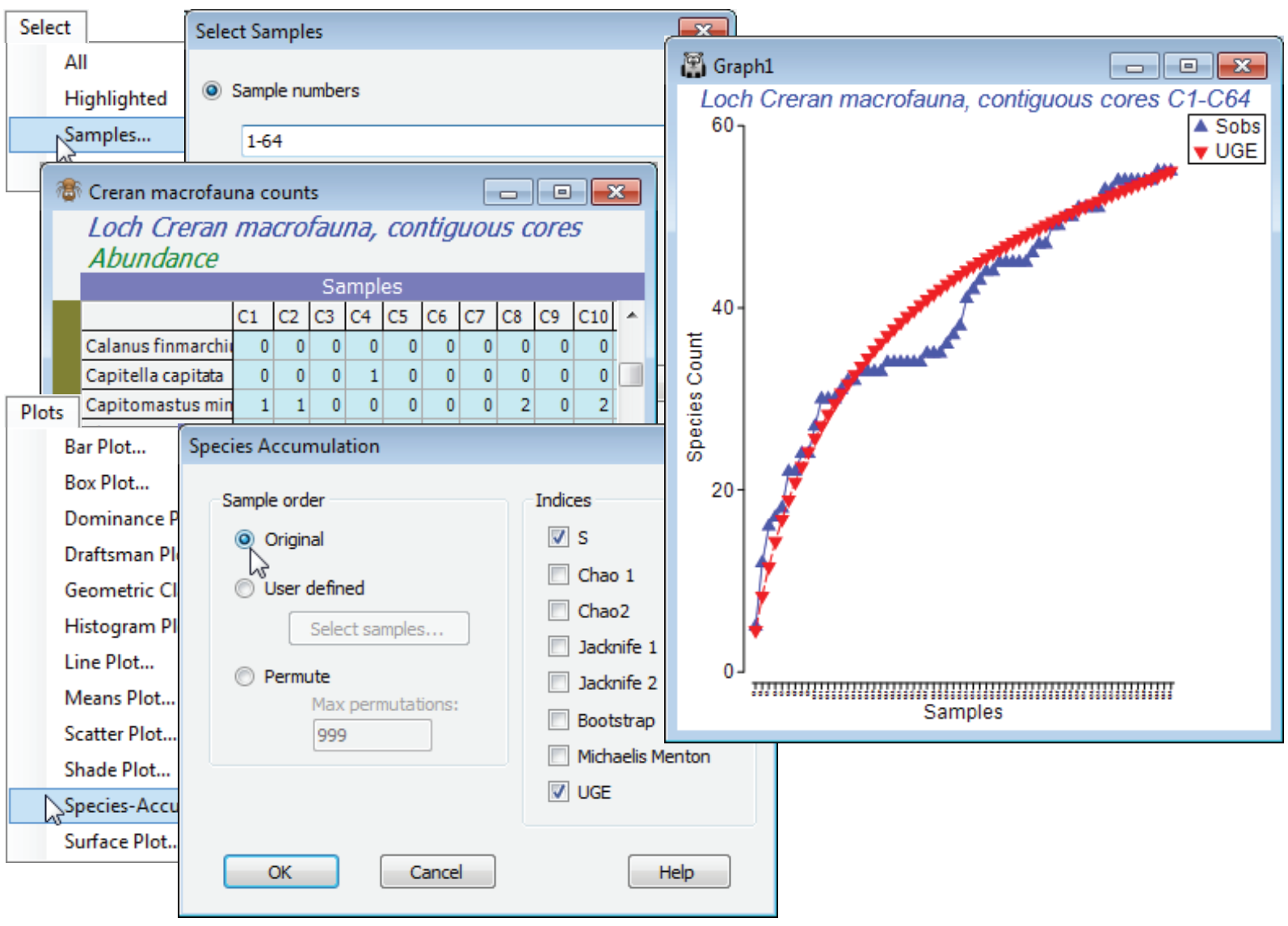
The analytical form of this mean value of the accumulation curve (over all permutations, in effect) was given by Ugland K, Gray JS, Ellingsen K 2003, J Anim Ecol 72: 888-897, and is computed by Plots>Species-Accum Plot>(Indices✓UGE). [It is the counterpart of the analytical form given by Hurlbert SH 1971, Ecology 52: 577-586, for the Sanders rarefaction curve met under Analyse>DIVERSE, which gave expected numbers of species for subsets of individuals from a single sample (whereas here we are talking about subsets of samples from a data matrix).] Although, for large numbers of permutations, the (✓UGE) curve will always lie on top of that from specifying (Sample order•Permute) & (Indices✓S), it is included as a separate option so that the combin¬ation of original sample order for S with the mean curve (UGE) can be taken. For samples that arrive in a non-arbitrary space or time order, this allows comparison of the real accumulation curve with its smoothed version – spatio-temporal heterogeneity will display as a jagged or stepped S curve.

Select the first 64 samples from Creran macrofauna counts, either using Select>Samples>(•Sample numbers: 1-64) or (•Factor levels)>(Factor name: sixtyfours)>Levels and Include only level 1, and submit to Plots>Species-Accum Plot>(Sample order•Original) & (Indices✓S✓UGE), unchecking the other indices. There is perhaps a suggestion of stepping in the S obs curve (though not much, and this would be hard to test for). However, it is clear that the accumulation curve is still rising and this raises the question as to how much larger S can get, with repeated sampling in this area.