Missing data estimation (Clyde study)
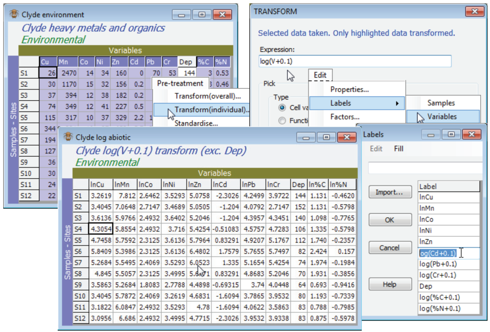
Transformation options for the Clyde environmental matrix, Clyde environment, are discussed in more detail in the following (PCA) section, but the tool to carry out separate transforms on sets of variables, Pre-Treatment>Transform(individual), rather than transforming the whole array, Pre-treatment>Transform(overall), was met in Section 4, applied to the environmental data from the Ekofisk oil-field study. Here, all heavy metals and organics (10 of the 11 variables) will benefit from log transformation, to reduce their right-skewness and so bring these continuous variables closer to normality across the sites (in so far as that can be judged from only 12 samples!). Thus, highlight all variables except Water Depth (Dep) and take Pre-treatment>Transform(individual)>(Expression: log(V+0.1)) & (✓Rename variables), renaming the result Clyde log abiotic. Give the variables in this sheet shorter names (e.g. lnCu, lnMn etc) with Edit>Labels>Variables.
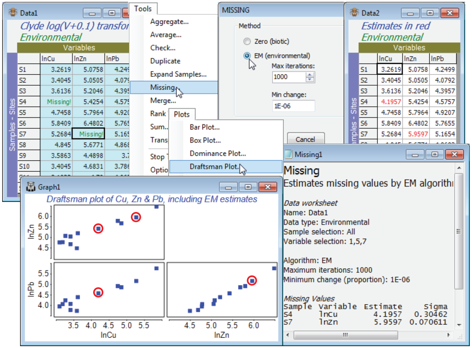
Take a copy with Tools>Duplicate and from this remove a couple of cells at random – perhaps (S4, lnCu) and hit the delete key, then (S7, lnPb) and delete again. Both cells will now be displayed as Missing!. Analyse>Draftsman Plot on this transformed data shows that normality assumptions are probably now acceptable (see the following section) but the above DpP criterion for the whole matrix fails badly (n = 12, p = 11, m = 2, so DpP = 1.7) and we should not trust the outcome even if Tools>Missing converges (it does not, here). The correlation matrix output with the drafts¬man plot does, however, show some very high correlations between e.g. Cu, Pb and Zn, which gives a better basis for prediction than the whole matrix. So, select just these three variables (highlight them then Select>Highlighted), and Tools>Missing produces credible missing data estimates of 4.18 (S4, ln Cu) and 5.26 (S7, ln Pb), compared with the original 4.31 and 5.17. Note that the ratio DpP = 3.3, which is still some way from respectability, but clearly is capable (sometimes at least) of producing useful results. The results window shows that the imprecision (under the assumption that the value is missing at random, of course) is lower for the estimated (S7, Pb) reading than the (S4, Cu) value, though both are rather well determined. The standard deviation of the estimate for (S7, Pb) is about 0.07 and for (S4, Cu) about 0.30, so that rough confidence intervals are (3.6, 4.8) and (5.8, 6.1) respectively. The reason for this difference in precision is clear from the draftsman plot for these three Cu, Zn, Pb variables, on which the respective points are manually circled (the plot window was copied and pasted to Powerpoint with Ctrl-C and Ctrl-V). The linear relationship between Pb and one of the other variables (Pb) is seen to be extremely tight, whereas Cu is not so highly correlated with either Zn or Pb, so there is inevitably greater uncertainty in the interpolation – it is a consequence of the multivariate normality condition that these relationships are estimated as straight lines. The estimates now need to be individually copied (click in the cell and Ctrl-C) and pasted back into the full matrix (Ctrl-V at the cursor). Of course the process is more automatic in less borderline cases, with larger n, when the full matrix can be input to Tools>Missing.


