Ordering by a worksheet variable
The core task faced by the Special>Reorder operation is to reduce what is inevitably a high-d similarity structure, on either axis, to a 1-d representation of those samples (or species). The default for Matrix display, when no group structure is provided for the samples, is to perform UPGMA (group average) clustering on the sample Bray-Curtis resemblance matrix, followed by optimising correlation to a seriation model matrix. So the Reorder dialog for the above will have Samples> (Order•Seriate & Sample resemblance Resema) & (Constraint•Sample dendrogram Graphb), with the same options for Variables (except based on group average clustering of Index of Association resemblances), but of course these are not the only possibilities. Any resemblance measure can be substituted on either axis, for the seriation, and any tree diagram for either dendrogram. We have seen the alternative of ordering by a numeric factor but (Order•Worksheet variable) also allows the sample axis to be ordered according to, for example, the value of an abiotic variable recorded over the same set of samples. This can be unconditionally or keeping samples from the same factor level together or only allowing rotations specified by a dendrogram – logically the dendrogram would be from the biotic matrix of the display. The latter is thus an interesting example of using both biotic and environmental data to produce a natural 1-d arrangement of samples not serially ordered by the biota. Apparent diagonalisation of the matrix can now be interpreted as a serial link between the selected environmental variable and the community pattern, without fear that we have ‘chased the noise’, since the sample clustering does not use the species order, or an internal seriation – instead it is the external abiotic variable that determines ordering (as opposed to grouping) of the samples.
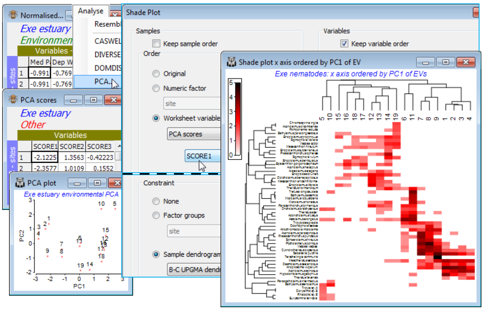
As an example, open Exe environment if this is not already in the workspace – this manual has not made much use of these 6 abiotic variables, recorded for all 19 sites, though see Fig. 11.7 in CiMC. A logical single summary variable of the abiotic pattern might be the first principal component PC1 from a PCA ordination (Section 12). Take Pre-treatment>Normalise Variables on Exe environment – there is no need for an individual transformation of any variables here – and Analyse>PCA>(✓Scores to worksheet) on the normalised matrix. The PCA plot shows that, if we were to use the first PC (SCORE1 in the sheet – renamed PCA scores – that this creates of the PCA co-ordinates), to order the samples in the shade plot unconditionally by this variable, we would not obtain a very meaningful sample order, either in terms of the (2-d) pattern of the biotic or abiotic samples – this is not a case of a single strong gradient (e.g. on PC1, site 10 would be split from 5 and placed in the middle of the loose 12-19 group). However, constraining by the existing biotic dendrogram (given by the original run of Matrix display) produces a neater, abiotic-driven dendrogram rotation, i.e. Special>Reorder>Samples>(Order•Worksheet variable PCA scores>SCORE1) & (Constraint• Sample dendrogram B-C UPGMA dendro) and (Variables✓Keep variable order). This last step greys out all the variable options and keeps the species list and dendrogram in the same order as above, avoiding a further 9999 seriation restarts – this can be useful in comparing sample options.

