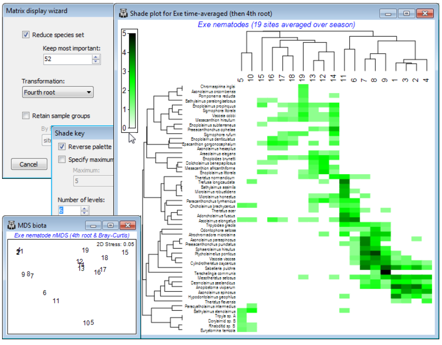
Clustering on species and samples (Exe nematodes)
The time-averaged Exe nematode community data were used extensively in Section 8 to illustrate nMDS ordination, and the workspace Exe ws in C:\Examples v7\Exe nematodes should contain the data sheet Exe nematode abundance of the 19 sites, averaged over the 6 bi-monthly sampling times. This data matrix is now an example where there is no a priori group structure on the samples (sites) so that it would be instructive to cluster both species and samples axes of the shade plot. It is also a case of clear (and almost complete) turnover in species among some groups of sites, contrasting markedly in a shade plot with the more subtle community changes seen for the Ekofisk macrofauna and Wrasse diets. There are many species here which are infrequently found and in low abundance, and a useful shade plot would concentrate on only the 50-60 ‘most important’, e.g. the analysis in Chapter 7, CiMC, picks only those species accounting for $\ge$5% of total abundance at any one of the 19 sites – using Select>Variables>(•Use those that contribute at least: 5 %) – which retains 52 of them. So, on the active matrix Exe nematode abundance, Wizards>Matrix display>(✓Reduce species set>Keep most important: 52) & (Transformation: Fourth root) and uncheck the (✓Retain sample groups) box. The plot needs little tidying up: you might wish to put more levels into the scale key by clicking on the key and (Number of levels: 6), and in order to match Fig. 7.7 in CiMC, you may also need to Flip X or Flip Y (accessed by Graph or right-click). The dominant pattern is one of strong diagonalisation of the matrix but there is a point to note here. In the previous cases, the order of the sample axis was fixed on external information (a physical gradient and an a priori group structure, with ordered categories), and only the serial order of the species axis was given by optimising a matrix correlation $\rho$ – but this seriation cannot be a function of the sample order since the species similarities would be unchanged by any sample re-ordering, hence observed diagonal-isation implies a genuine gradient effect. When both axes are seriated as here (subject to constraints imposed by dendrogram rotation) then we need to be more careful in interpreting diagon¬alisation – it is inevitable that if both axes are internally ordered to an optimum degree, then the combination of them must appear diagonal¬ised, at least to some extent. In fact, the nMDS configuration (Section 8) is not that of a simple linear gradient. Though the primary species in site group (5,10) could be rotated manually (by clicking on the dendrogram bar of the last species grouping) to sit at the top left rather than bottom left corner, this is arbitrary. The group is close to having an exclusive set of species – this would have made it 100% dissimilar to everything else and able to be placed at either end of the sequence (or even in the middle, if there were other sets of mutually exclusive species).

