Pairwise comparisons

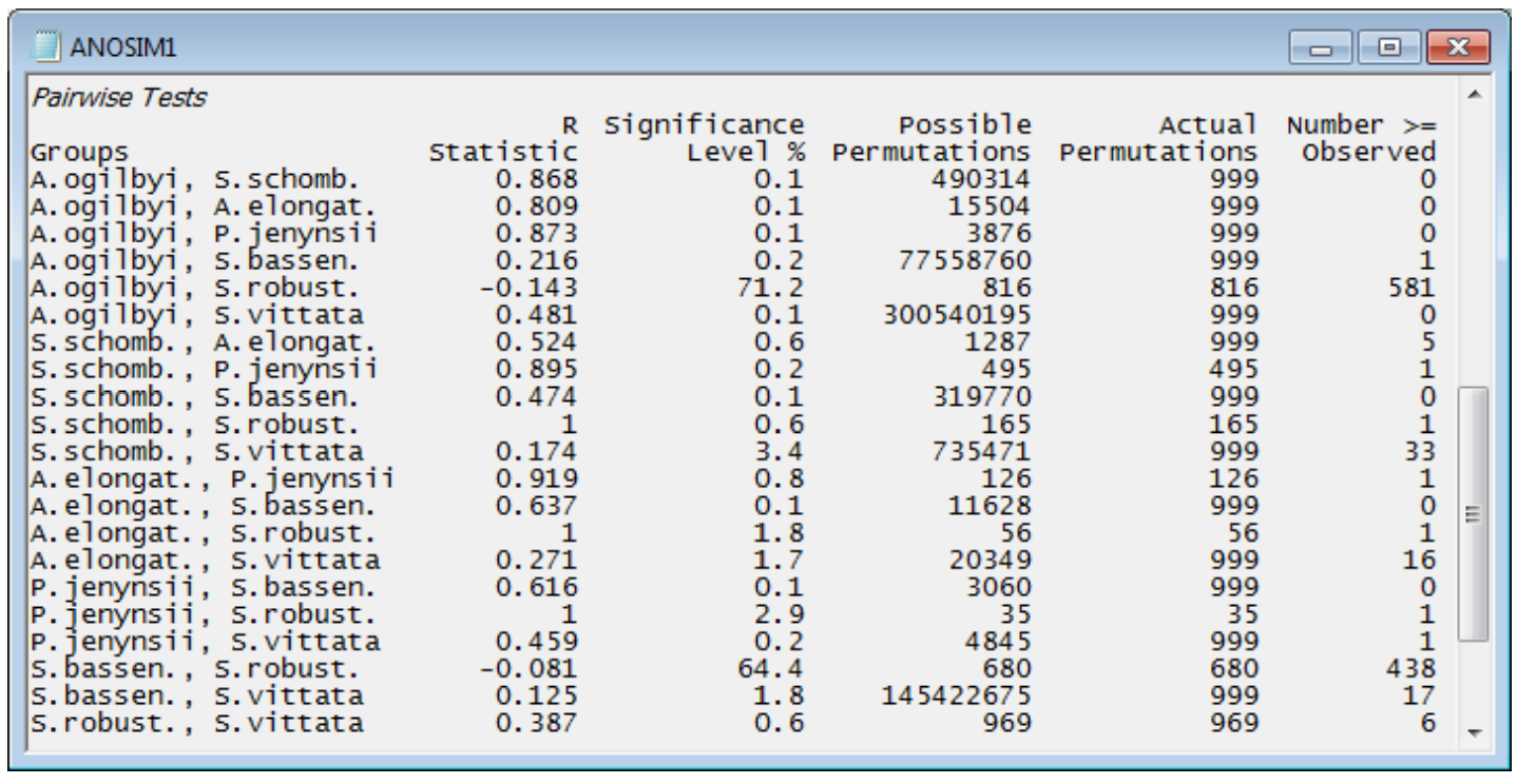
The table ending the results window gives the pairwise comparisons. For each pair of groups (fish species), the first data column is of pairwise R statistics. These are again a difference of average rank dissimilarities between and within the two groups, scaled so that R varies between roughly 0: there are no differences, and 1: all dissimilarities between gut contents of different fish species are larger than any dissimilarity among samples within either species. The second column gives the statistical significance for a test of R = 0 (again as a percentage, so that p<0.1% means less than a 1 in 1000 chance). The number of possible permutations follows, then the number actually computed – 999 in most cases because the possible number is usually much larger than this, here. The final column gives the number of R values from the permutations that exceed (or equal) the real R in the first column, from which the significance in column 2 is calculated. [Note that there needs to be a slight difference in this computation depending on whether all possible permutations are evaluated. Thus row 1: A. ogilbyi v S. schomb., R = 0.868, p<100(1+0)/(1+999) = 0.1%, whereas row 12: A. elongat. v P. jenynsii, R = 0.919, p = 100(1/126) = 0.8%. The second is clearest: the observed value of 0.919 is the most extreme of 126 permutations and thus has probability 1 in 126 of occurring by chance. In the first case, we do not observe the real value of 0.868 in our randomly chosen set of 999 permutations, but that does not make the probability p = 0/999 = 0. We know there exists one permutation which would give R at least 0.868 – the real configuration – and we have looked at 1000 permutations overall (the 999 random plus the real one) so the probability is < 1 in 1000.]

Interpreting these pairwise tables must be done with care. The significance level is very dependent on the number of replicates in the comparison. For example, row 4: A. ogilbyi v S. bassen., p<0.2% (your value may differ slightly because each time the routine is run, different random permutations will be generated). This appears highly significant, but the R value is negligibly small, at 0.216. The test tells us that these two species probably do not have exactly the same diet (the hypothesis R = 0 can be rejected) but the R value tells us that the diets are strongly overlapping and barely differ (R is close to zero). This can happen, just as in ordinary univariate statistics, because the number of replicates is large for the two groups, giving 77 million possible permutations – biologically trivial differences can still be statistically significant when the test’s power is large. In total contrast, row 17: P. jenynsii v S. robust., p<2.9%, still significant but only just (at the 5% level), has an observed R of 1.0, the largest possible value, which shows completely different diets. Such a large value of R does not give a small value of p because there are only 35 possible permutations (few replicates in both groups). Which is therefore the most useful column to interpret? It has to be the R values and not the p values. R is largely not a function of the number of replicates (i.e. possible permutations) but an absolute measure of differences between two or more groups in the high-dimensional space of the data, whereas p is always hijacked by the sample size. It is for this reason that PRIMER does not implement a Bonferroni-type correction on its pairwise significance levels – it gives an illusion of certitude which is not justified. The global test of any differences between groups is important: if the null hypothesis is not rejected then the user has no licence to look at the pairwise comparisons. However, if the global test strongly suggests that there are differences worth examining, the focus shifts to the pairwise R values – large values there indicate where the major differences are found.