Linking MDS plots to cluster analysis

The 2-d ordination plot shows a clear separation of the nematode assemblages at these 19 sites into 5 groups (which CiMC, Chapter 11, shows can be related to sediment properties such as the median particle size, anoxic layer depth and interstitial salinity). Another useful check on the adequacy of the 2-d approximations represented by both MDS and cluster analyses, to the real high-d structure (there are 140 species variables in the Exe nematode abundance data sheet!), to examine the MDS and dendrogram results in combination, and there are at least two ways of doing this.

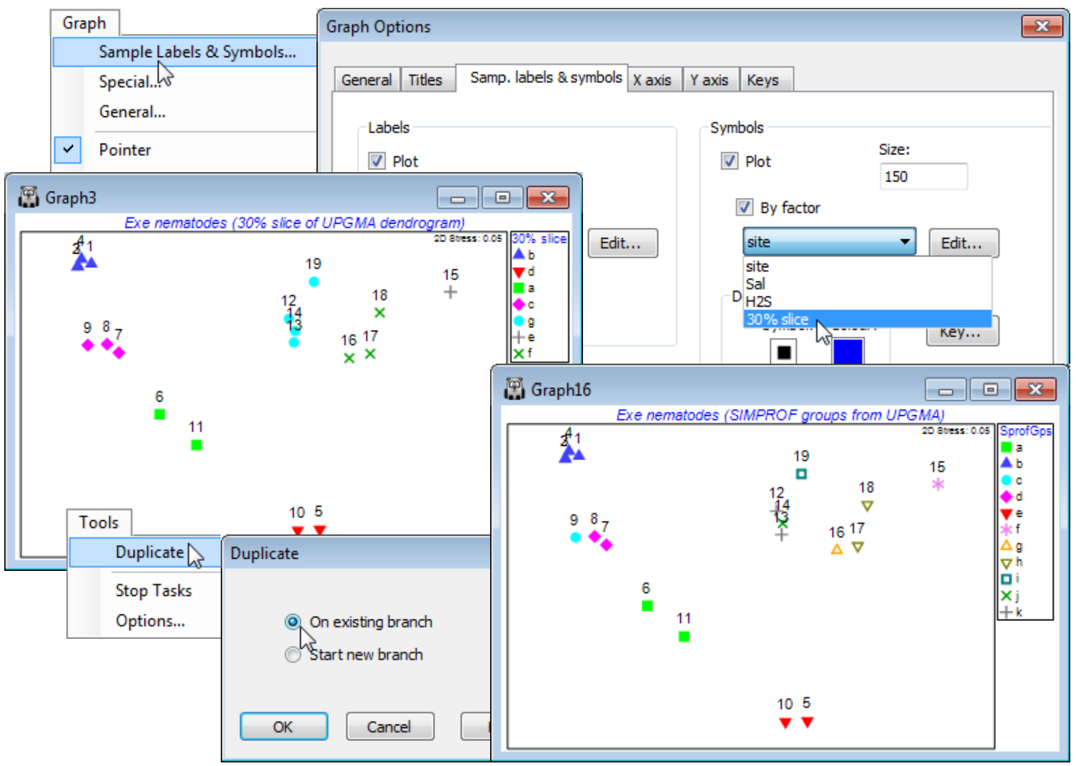
Firstly, the clusters that are defined for a fixed similarity slice through the dendrogram can be put into a factor, with levels defining the different groups, as seen in Section 6. This factor can then be displayed as differing symbols on the MDS, and the agreement noted. A variation of this which may often be preferable is to use the factor (or factors) created by the series of SIMPROF tests which accompany the particular clustering method (or methods), defining group structures for which there is some statistical support. For the current Exe ws workspace, a similarity slice should already exist as the factor 30% slice from the dendrogram Graph1. (If not, recreate it, with Graph1 as the active window, by Graph>Special>Slicing:(✓Show slice)>(Resemblance: 30) & (Create factor>Add factor named: 30% slice). From the MDS (Graph3), take Graph>Sample Labels & Symbols>(Symbols✓Plot)>(✓By factor: 30% slice) & (Labels✓Plot)>(✓By factor: site). (When plotting both labels and symbols, note that the symbol is centred on the point, with the label above. On its own, either is correctly centred). You might also like to re-run the Analyse>Cluster routine on Resem1, for one of the clustering methods discussed in Section 6, defining SIMPROF groups by a factor which is again used as symbols on the MDS. (Use Tools>Duplicate>(•On existing branch) on Graph3 to create a copy of the MDS so you can juxtapose the differing factor selections. You may also want to re-order the key by clicking on it and using and repeatedly in the resulting Key dialog). You will see that a finer distinction of sites into clusters is obtained with SIMPROF, implying there is statistical evidence for interpreting such fine-scale groups – but the ability to slice the dendrogram at some arbitrary coarser similarity (or to define fewer groups with the flat-form clustering, kRCluster) may still be a justifiable approach for a practical application of site grouping.

A good example of the comparison of different clustering methods and the SIMPROF groups they generate is seen in CiMC, Fig. 3.10, for the zooplankton data in the Bristol Channel ws workspace. Section 6 produced a range of SIMPROF factors: SprofGps, Flexbeta, Single & Complete linkage (agglomerative hierarchical), Unctree (divisive hierarchical) and Flat R (flat-form) clusters, which you may wish to represent as symbols on duplicated MDS plots, in a similar way to the above.