2STAGE for resemblance coefficients (Clyde study)

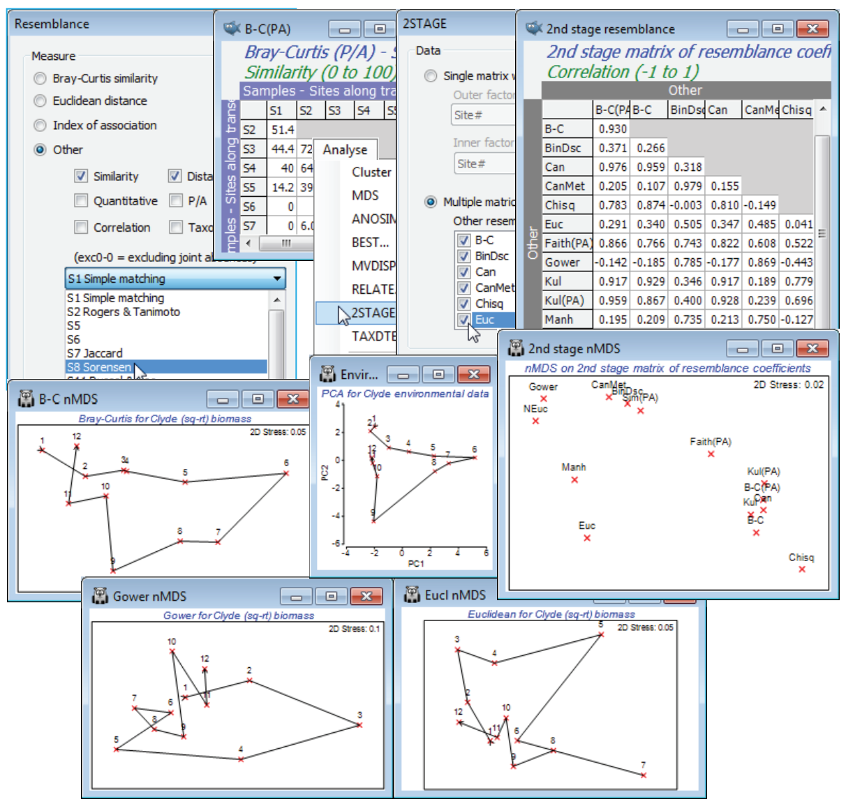
The technique of 2nd stage plots has also been used (Clarke KR, Somerfield PJ, Chapman MG 2006, J Exp Mar Biol Ecol 330: 55-80) to examine the effects of different resemblance coefficient choices on a samples analysis, scaling this in relation to the effects of differing transformation (and, by extra¬polation, taxonomic level). The environmental data from the Clyde sewage dump-ground study were used extensively in Sections 11 and 12 but, for this example, open the macrofaunal data C:\Examples v7\Clyde macrofauna<ins>Clyde macrofauna biomass into a new workspace, and deselect the all-blank species (there are about 20 of them retained in this sheet because they have non-zero counts in the abundance matrix but their total biomass is too small to weigh). You can do this by Select>Variables>(•Use those that contribute at least 0.001%), then take a square-root transform (Biomass sq-rt). Always starting from this matrix, produce a wide range of distances and (dis) similarities using Analyse>Resemblance>(Analyse between•Samples) & (Measure•Other)> (Similarity) & (Distance/dissimilarity), selecting one coefficient at a time from the resulting list, e.g. S1 Simple matching, S8 Sorensen (i.e. Bray-Curtis P/A), S13 Kulczynski (P/A), S26 Faith (P/A), S15 Gower, S18 Kulczynski (quant), Canberra similarity exc 0-0, D7 Manhattan distance, D10 Canberra metric, D16 Chi squared distance, Binomial Deviance (scaled) and (•Bray-Curtis similarity) and (•Euclidean distance) from the main dialog, the latter both with and without normalisation of the species variables. [You should read the discussion in Section 5 and in Chapter 16 of CiMC on the suitability or otherwise of some of the coefficients in the full list, for non-count data]. With (say) S8 Sorensen as the active sheet, Analyse>2STAGE>(Data•Multiple matrices), ticking the check boxes for all the rest, and running nMDS on the resulting 2nd stage matrix. Look also at individual MDS plots for some measures with differing effect, in comparison with the contaminant gradient (the multivariate analysis for which – a PCA – is shown in Section 12). Crosses have been used for points in these plots, by changing the symbol type temporarily in the Samp. Labels & Symbols>(Default>Symbol:) dialog or, changing the global default by Tools>Options>Graphs.