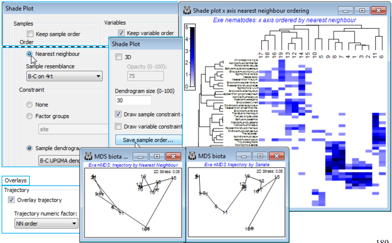
Nearest neighbour ordering

The final option that Reorder offers, attempting to find a useful ordering on a 1-d axis of a non-serial structure, is (Order•Nearest Neighbour) which implements a simplified travelling salesman algorithm. This is available for both samples and species axes, and an example where it is applied to both axes is seen in Fig. 7.9 of CiMC, but here for the Exe nematode data we shall run it on the sample axis only, again keeping the species order the same with (VariablesKeep variable order). The full travelling salesman problem would be to find a route through the samples in which all are visited just once, and which minimises the total ‘distance’ travelled – in this context that means minimising the total dissimilarity between adjacent pairs of samples when placed in that order. We saw something similar with the minimum spanning tree in Section 8 (see box heading for MST), for precisely these Exe data. However, as the nMDS there shows, an MST allows branching of the route and this does not then provide a unique 1-d order in which to place the samples – but that plot does illustrate the point that a travelling salesman route should be greatly superior to, for example, taking the first axis of the 2-d MDS plot, when sites 5 and 10 would be interpolated in the 12-19 group (thus with unhelpful sample order in the shade plot of …, 12, 14, 13, 10, 19, 5, 16, …). The full travelling salesman problem is numerically highly demanding (a so-called NP-hard problem), even for modest numbers of samples, and PRIMER 7 currently implements the ‘greedy’ travelling salesman algorithm (see Chapter 7, CiMC), which is not an iterative process – so runs quickly – but may find an acceptable route, albeit possibly not an optimal one. It involves successive joining of nearest neigh¬bours to one or other end-point of the route, hence run by (Order•Nearest Neighbour).

For the existing shade plot of the Exe nematode data, Tools>Duplicate it (on the existing branch) and run Special>Reorder>Samples>(Order•Nearest neighbour>Sample resemblance B-C on 4rt) & (Constraint•Sample dendrogram B-C UPGMA dendro) and (Variables✓Keep variable order). The B-C on 4rt sheet is just the sample resemblances from the Matrix display run, used for all these shade plots – Bray-Curtis on 4th root transform of the nematode abundances, using the full set of species, which also gives the clustering B-C UPGMA dendro. You may need to Flip X to obtain the shade plot below. To note the order in which (•Nearest Neighbour) places the sites in relation to their (non-serial) pattern in the 2-d nMDS, on the shade plot take Special>Save sample order>(Factor name for sample order NN order), thus creating a factor which you can import (if necessary) into any sheet on the branch of the nMDS, with Edit>Factors>Import. On MDS biota, the 2-d nMDS, take Graph>Special>Overlays>(✓Overlay trajectory) and supply NN order. If you repeat this for the original serial order factor, the difference between ordering samples across the plot (•Seriate) or along a winding trajectory (•NN) is clear – and seen more starkly still in Fig. 7.9, CiMC – but the constraints imposed by the cluster analysis make either of these solutions better 1-d orderings for the purposes of shade plots than use of the first axis from a 2- or higher-d ordination. (Note that a 1-d MDS is not offered in PRIMER since each restart is sure to get trapped in a local minimum of the stress – there is limited ability to move points past each other in iterations in 1-d ).