Accuracy & fit scheme
For the MDS run above, two of the defaults taken for options in the MDS dialog were (Minimum stress: 0.01) and (Kruskal fit scheme•1). Changing the former from 0.01 to 0.001 would decrease the lower threshold of stress at which the iteration decides that it has effectively reached a perfect solution but, more usefully, also increases the accuracy with which stress values are reported in the results window. Reporting stress to a third decimal place can be useful in deciding whether a batch of restarts with the same stress, to two decimal places, are really the same solution. However, it is unwise to take small differences in stress too seriously: solutions with nearly the same stress will usually lead to the same interpretation. A low-dimensional ordination is only an approximation to the real high-dimensional pattern, in any case, and not necessarily a very good one. (This is the reason that most of the substantive analysis, like hypothesis testing, takes place on the resemblance matrix and not in a low-d ordination space. It therefore misses the point to worry unduly about whether a low-d plot is the optimum placement of the points or one that is very nearly optimal – both are only approximations to the truth). In fact, it can be quite revealing to look at repeat MDS runs with only one restart, which much of the time will therefore converge to an inferior solution, and observe which points differ from their placement in the optimal solution.
The (Kruskal fit scheme•1) option is by far the commonest choice for practical nMDS. Essentially, it allows dissimilarities which are equal (tied ranks) to be represented in the final ordination by distances which are not equal, whereas (Kruskal fit scheme•2) constrains those plot distances to be equal. The latter can be an unhelpful constraint in any situation in which there is a complete turn-over of species across some samples. For example, along a strong environmental gradient, such as water depth say, there could already be complete species turnover in benthic organisms between sedimentary sites at 5m and 100m (dissimilarity = 100%), but two sites at 2m and 200m, or at 1m and 500m, cannot give a larger dissimilarity than this. If 100% dissimilarity is to be represented by exactly the same distance in the ordination of samples widely spread along this depth gradient, it is inevitable that an arched (or to be more precise, staple-shaped) solution will result from what is actually a strong linear gradient. This is one of several explanations for the arch effect seen in other ordination techniques (such as PCO), to which nMDS is less prone because of the flexibility under (Kruskal fit scheme•1) to represent the set of 100% dissimilarities by different plot distances.
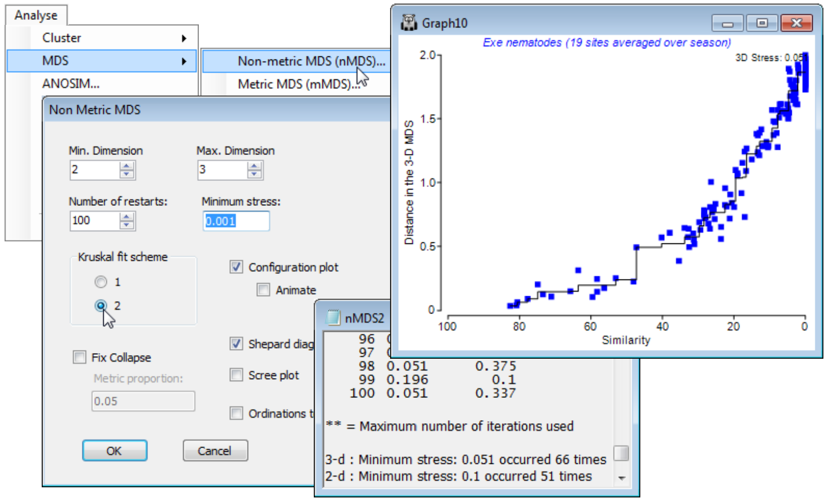
The above Shepard plots for the Exe nematode data – which is an example of large-scale species turnover – show this flexibility, in representing the many similarities of zero (dissimilarities of 100) by distances from about 1.6 to 2.4 in the 3-d plot, with stress of 0.033 (when run to 0.001 accuracy). Re-running for (Kruskal fit scheme•2) is seen below to force these distances closer to equality (1.8 to 2) and slightly degrades the solution (stress = 0.051 for the 3-d plot). The extra d.p. in quoting stress has not here demonstrated much of a spread of near-optimal solutions at a finer scale: the lowest stress of 0.051 is obtained at only a little lower frequency than before (66 of 100).

