Special menu for divisive trees

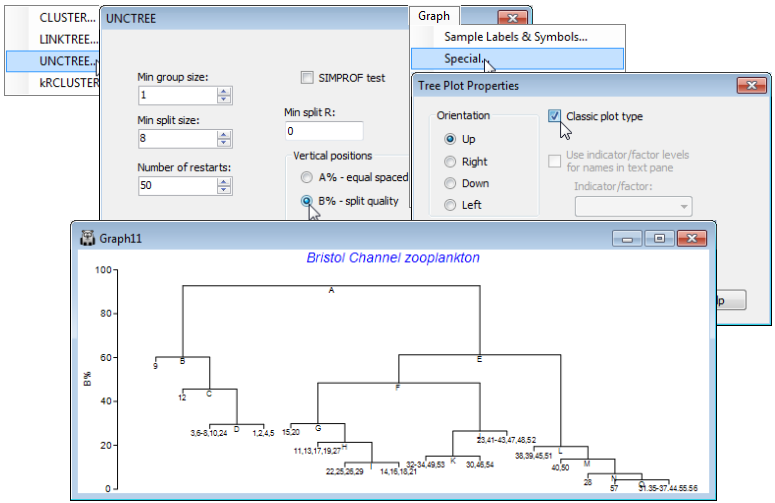
PRIMER 7 also provides a choice of representations of the tree structure, using either the A% or the B% axis scale. In general, the layout shown above is to be preferred, because the regular spacing of the sample axis allows non-numeric labels and/or symbols to be added, exactly as for a CLUSTER dendrogram. However, the Clarke et al 2008 paper used the tree layout shown below, referred to as classic format, an option from the Special menu, and this may still occasionally be found useful. Re-run the divisive clustering, this time with Analyse>Cluster>UNCTREE>(Min group size:1) & (Min split size: 8) & (Number of restarts: 50) & (Min split R: 0) & (Vertical positions•B% – split quality), unchecking the (✓SIMPROF test) box this time. On the right-click menu, when over the plot, take General and uncheck (✓Show text pane), setting (Overall font scale: 140), then Special> (✓Classic plot type). The other options on this Tree Plot Properties dialog are not relevant here. In the standard plot mode they would allow the tree to be shown on its side or inverted (as seen earlier for the equivalent Special menu for a dendrogram from CLUSTER), and the greyed out option is only applicable to the constrained form of this divisive clustering (LINKTREE), where explanatory variable names (e.g. environmental) are given as inequalities in the text pane, and it is convenient to expand or abbreviate the names using an indicator defined on those variables, see Section 13.

Two features are apparent from this plot. Firstly, the use of B% scaling on either type of plot does show (as a dendrogram would) that the divisions lettered A , E, F are major divisions between the clusters, in relation to the subdivisions of those groups, e.g. at H, J, L etc at much lower levels on the y-axis scale; this fact is missing with the equi-stepped A% scale. However, there is the potential for reversals when using B% scaling (sub-cluster divisions returning higher values of B than their parent split) especially in the constrained form of this clustering (Section 13). Secondly, note that labels on the ‘classic’ plot have to be sample numbers, exploiting number ranges to keep the plot tolerably neat (text labels would be impossible), which is highly confusing here when the sample sites are actually labelled 1-29, 31-58 (site 30 not sampled), but the sample numbers will be 1-57!