(Leschenault estuarine fish, W Australia)
Veale L et al 2014 J Fish Biol 85: 1320-1354 describe trawl sampling for nearshore estuarine fish in the Leschenault estuary of Western Australia, over 4 regions (B - Basal, L - Lower, U - Upper, A - Apex of the estuary) and 4 seasons (Sp - Spring, S - Summer, A - Autumn and W - Winter). The data set used for this illustration has been somewhat simplified and consists of 6-8 replicate 21.5m seine net samples reflecting both inter-annual and spatial variation within each of the 16 regionseason combinations. Due to the location of freshwater inputs and restricted exchange with the ocean, the estuary has a salinity gradient which increases from the basal (mouth) through lower and upper regions to the estuary apex. Counts are given of 43 fish species (with numerical ID), file Leschenault fish counts in C:\Examples v7\Leschenault fish. Close the above workspace and open this file, with factors Season and its (0, 1) numeric form Cycle (0, 0.25, 0.5, 0.75), then Region.
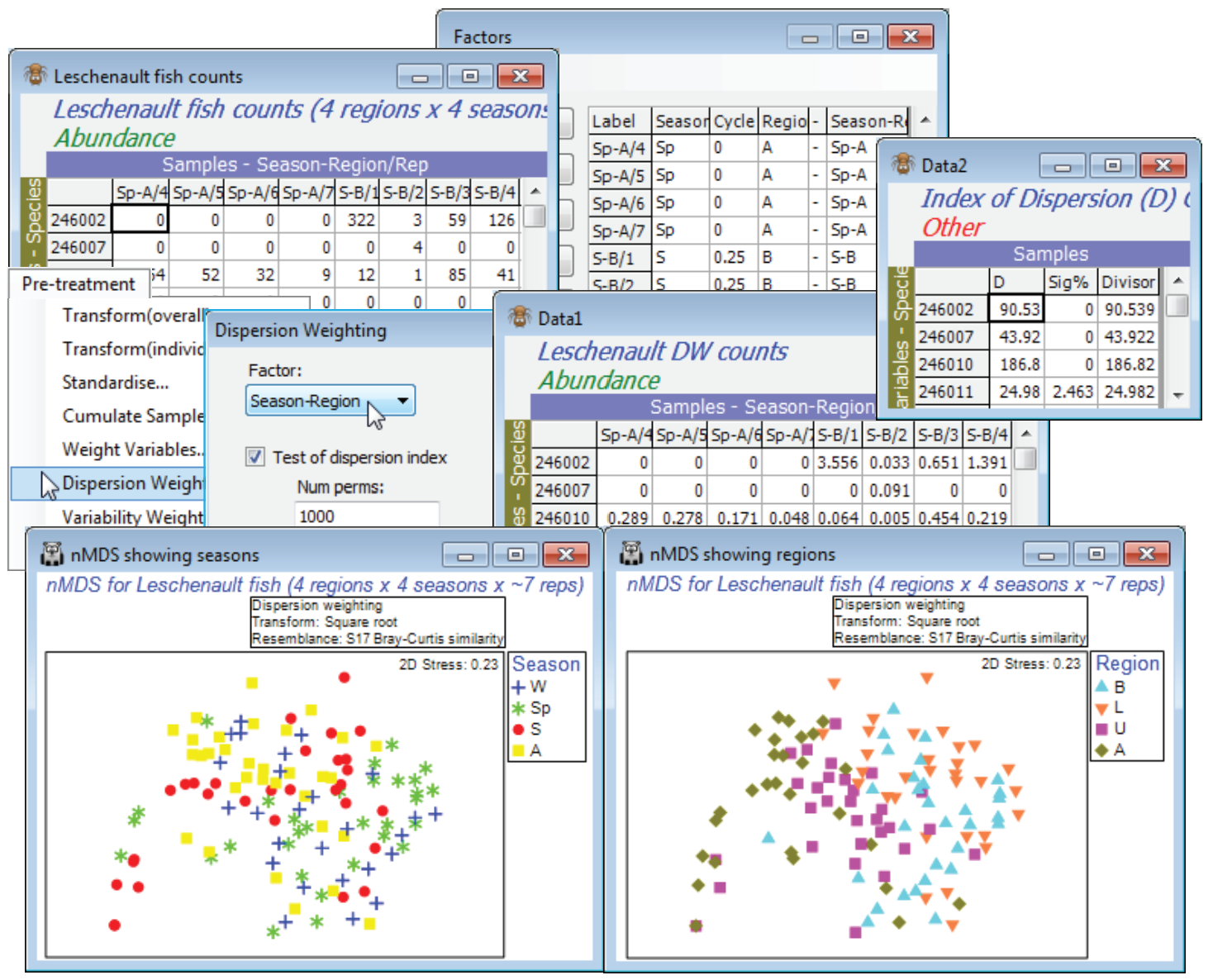
As often with fish data, over-dispersion of counts (shoaling) can be substantial for some species, their erratic counts over replicates giving them too much weight in a community assessment, and Clarke KR, Tweedley JR, Valesini FJ 2014 J Mar Biol Ass UK 94: 1-16 show that a good strategy for such fish data is often pre-treatment by Dispersion Weighting (Section 4 and Chapter 9, CiMC) followed by mild transformation (square root). So, take Edit>Factors>Combine>(Include: Season & - & Region), where - is just a hyphen separator in all rows, to create a new factor Season-Region whose levels identify the groups of replicates from the 16 conditions. Use this in Pre-treatment>Dispersion Weighting>(Factor: Season-Region) & (✓Test of dispersion index) &(✓Stats to work-sheet), and the latter sheet shows that counts of some species are, indeed, heavily downweighted by an index of dispersion D of up to nearly 200. However, Plots>Shade Plot (Section 4) or Wizards> Matrix display (Section 10) on the dispersion-weighted data still show that the contributions to the resemblance matrix will come from relatively few of the species, so take a further Pre-treatment> Transformation(overall)>(Transformation: Square root). Now calculate Bray-Curtis similarity on this full set of 119 samples (B-C on root DW), and an nMDS ordination with symbols for Region, and duplicated with symbols for Season, show a great deal of replicate variability and consequent high stress, but also some evidence for effects of both factors.
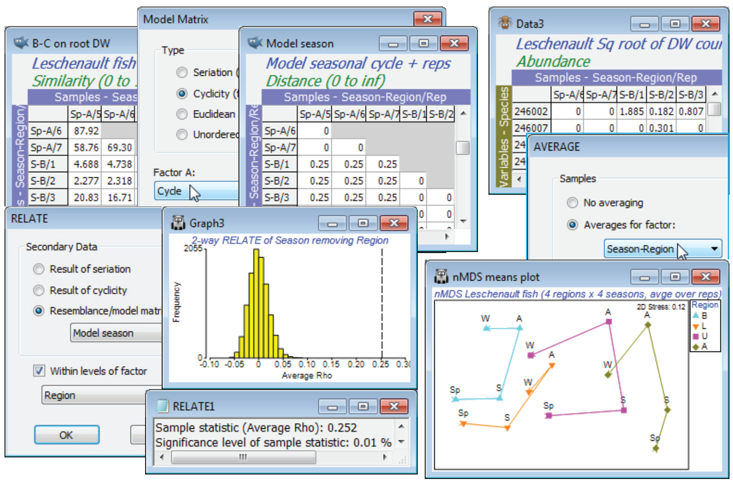
Unordered two-way ANOSIM with factors Region and Season is perfectly viable and will provide pairwise comparisons, though there is a good case for 2-way ANOSIM with an ordered Region factor, because of the salinity gradient and the geographical ordering of the regions B, L, U and A (note that a numeric factor would need to be created to capture this order). Such a serial order is not appropriate for Season, however, with the cyclic relationship of its levels (the factor Cycle, with Sp = 0, S = 0.25, A = 0.5, W = 0.75; though Sp could equally well have been coded 1, of course). The optimum test of Season therefore creates a model structure from B-C on root DW with Tools> Model Matrix>(Type•Cyclicity) & (Factor A: Cycle) to give Model season and tests it by 2-way RELATE on the active sheet B-C on root DW with RELATE>(Secondary data•Resemblance/ model matrix: Model season) & (✓Within levels of factor: Region). The resulting match to a cyclic seasonal pattern in each region – under the 2-way model, separately calculated then averaged to give $\rho$ = 0.25 – is low but this simply reflects the high replicate variability and therefore the strong overlap of the communities in the different seasons for the same region. Importantly, this value is highly significantly different from zero, as the histogram shows (p<0.01% since 9999 permutations were again used). This certainly justifies an nMDS means plot, averaging the replicates for the 16 conditions (4 seasons $\times$ 4 regions). As we have seen, there are several possible ways to do this – averaging the replicates of the original counts, or the dispersion weighted and transformed data, or the similarities (or, in PERMANOVA+, using distances among centroids in the high-d PCO space). Here, take the second method, Tools>Average>(Samples•Averages for factor: Season-Region) on the transformed DW data matrix, then recalculate the Bray-Curtis similarities and the nMDS, on which display symbols as Region as labels as Season using Samp. Labels & Symbols, and overlay split trajectories using Special>Overlays>(✓Overlay trajectory:Cycle)>(✓Split trajectory:Region). Both the consistent community change up the estuary (B,L,U,A) and the matching seasonal cycles are evident. (Lines logically joining W and Sp, as in Fig. 15.12 of CiMC, can be added by copying and pasting the plot into Powerpoint, or similar software, where it can be ungrouped to Microsoft drawing objects and manipulated as vector graphics). Close the Leschenault workspace.


