Aggregation

So far we have only seen variable information sheets, containing taxonomic (or other) hierarchies (*.agg files), used in calculating specialised forms of resemblance which exploit the relatedness of species in the samples being compared (Section 5). More significantly, this idea of relatedness or distinctness, as expressed in the variable information of the whole taxonomic tree, is the basis of a suite of biodiversity measures (Section 15). But the nomenclature of aggregation file (*.agg) comes from the original use of such taxonomies simply to aggregate up an abundance (or other) species matrix to, for example, genus level, i.e. to create a matrix of the abundances that would have been recorded had the species only been identified to a coarser taxonomic accuracy. There are several reasons for wishing to do this, e.g. the taxa might be thought too prone to mis-identification at the species level. Perhaps the data matrix was created over time by several taxonomists with differing expertise in particular taxonomic groups – a ‘lowest common denominator’ taxonomic level would then certainly lead to a more robust multivariate analysis. Alternatively, the motivation might be resource-driven – if it is possible to establish a putative environmental impact through community change just as clearly with a family-level as a species-level analysis then routine monitoring for that type of impact might be more cost-effectively carried out with data identified to the coarser level. Chapter 10 of CiMC gives many practical comparisons of species- and higher-level analyses.

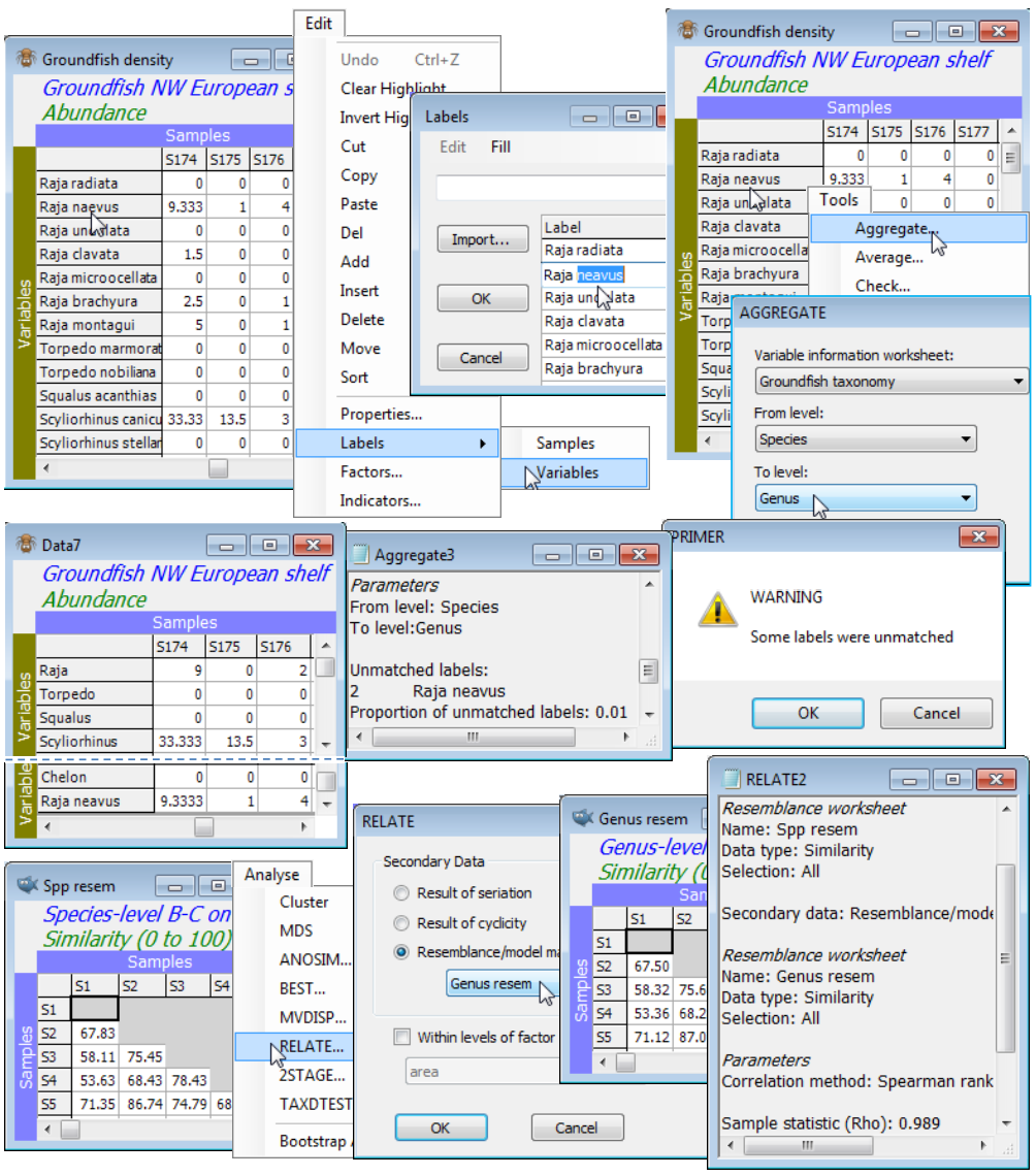
Whilst, as noted above, pooling the entries for species subsets, separately for each sample, could be accomplished by setting up an indicator and using Tools>Sum, this is more conveniently carried out with Tools>Aggregate. This works on the original data sheet (prior to any transformation) and specifies a variable information (aggregation) sheet and the hierarchical levels between which the aggregation needs to take place. Of course, unlike data and resemblance matrices the aggregation sheet is not restricted to numeric entries – its variable labels will typically be full species binomial names, and the subsequent columns the increasingly higher level (genus, family, order etc) names. The advantage of pooling using Aggregate is that the variable information file of the taxonomic (or other) hierarchy can be a look-up table which applies to a wide range of different data sets. There is no necessity for it to have the same number of species, or for those species to be in the same order, as in the data matrix, as long as all the data matrix species can be found in the more comprehensive faunal list which constitutes the aggregation sheet. Correct (or at least consistent!) spelling is thus essential, including spaces, periods etc. If a species name is not found, a warning is displayed, the results window lists which names were not matched, and these species are retained – with the same values – and with their species name being the higher-level variable name in the aggregated matrix.

Groundfish density and Groundfish taxonomy should be open in the current workspace. In this case the two sheets have the same full list of 93 species in the same order. With Groundfish density as the active window, Tools>Aggregate>(Variable information worksheet: Groundfish taxonomy) & (From level: Species) & (To level: Genus), pools the densities to a sheet which you should rename Groundfish genera. Square-root transform both data sheets and compute Bray-Curtis similarities. There is little point in trying to compare the nMDS ordinations for the two cases since the large number of samples (277) makes 2- (or 3-d) representations inadequate (high stress). But Sections 13 & 14 make much use of the idea of non-parametric correlation of resemblance matrices, e.g. with the Analyse>RELATE routine giving a measure of agreement in representation of sample relationships. Running this on the species and genus similarities gives a high level of agreement, $\rho$=0.989. You might like to start the example by mis-spelling a species name (e.g. Raja neavus) to observe the consequences, then change it back before running the comparison.