(Messolongi diatoms & abiotic data)
A study of diatom assemblages (abundances of 193 species) at 17 sites in the lagoons of Messol-ongi, Aitoliko and Kleissova in Eastern Central Greece was undertaken by Danielidis DB (1991), Ph.D. thesis, Univ Athens. At each site, a suite of 11 water-column data was also recorded: Temperature, Salinity, DO$_2$, pH, PO$_4$, Total P, NH$_3$, NO$_2$, NO$_3$, Inorganic N and SiO$_2$. The data files are Messolongi diatom density and Messolongi environment in C:\Examples v7\Messolongi diatoms. This is an ecological study of how the diatom communities relate to the water-column variables.
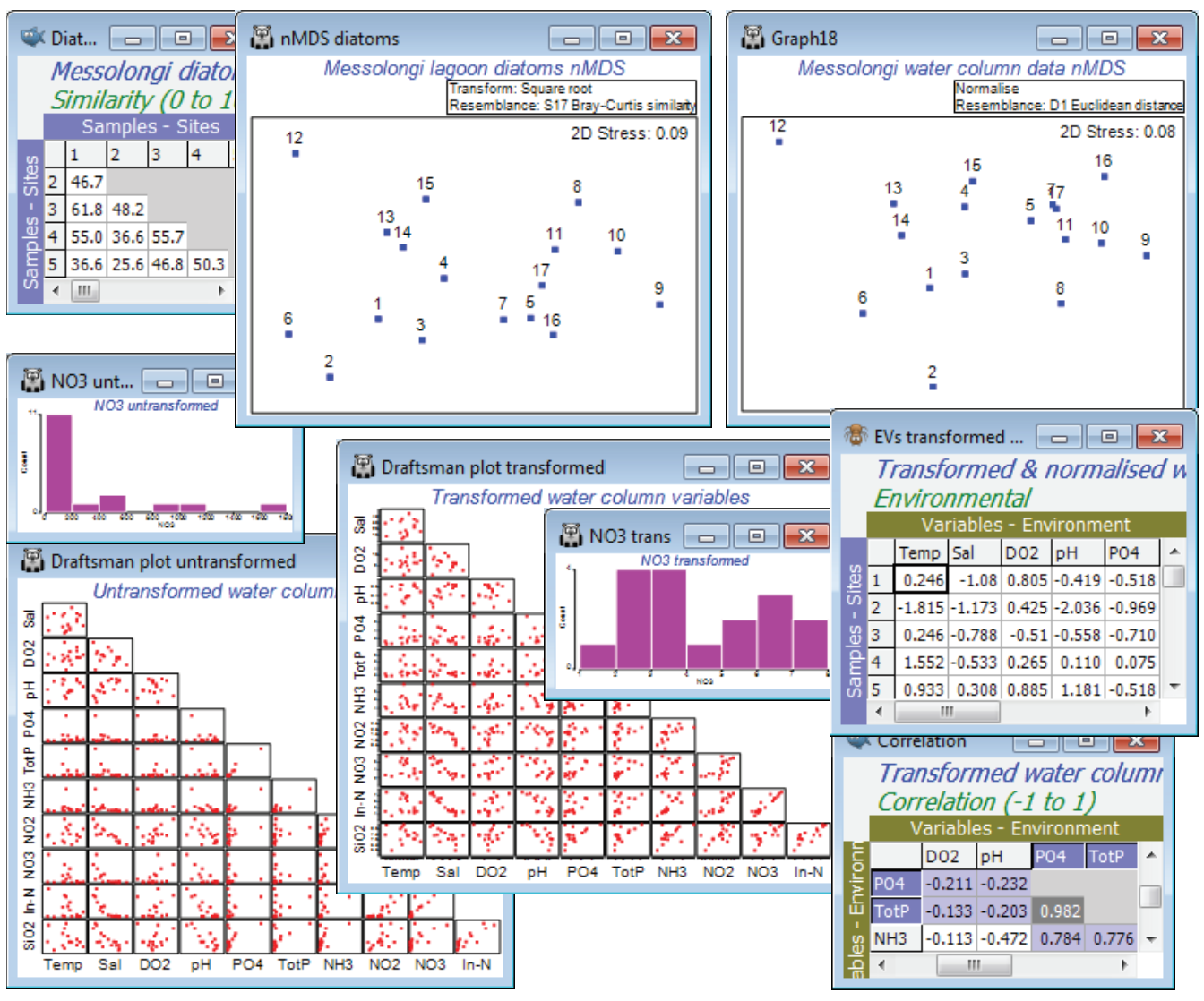
Square-root transform the abundance file and take Bray-Curtis resemblances, plotting the nMDS as usual. Plots>Draftsman Plot or Histogram Plot show that a log transform would be desirable on the nutrient concentration variables PO$_4$, TotP, NH$_3$, NO$_2$, NO$_3$, In-N and SiO$_2$, but Temp, Sal, DO$_2$ or pH do not need any transformation. As in the previous section, carry this out by highlighting (not selecting) the variables to be transformed and take Pre-treatment>Transform(individual)>(Expression: log(V)), unchecking the (✓Rename variables) box – readability of the BEST output is improved if not all the variable names look like log(...)!, so bear in mind that PO$_4$ means log(PO$_4$) etc, from now on. Re-running Draftsman and Histogram Plots, and also taking (✓Correlations to worksheet) for the former, shows that the distributions now have greatly reduced right-skewness. Two variables, PO$_4$ and TotP are seen to be strongly collinear, and it will make sense to drop one of them in the BEST run – they are, in effect, the same variable. You can pick out which are the very strongly correlated variables by Select>Samples>(•Values>0.95) on the correlation matrix produced by the draftsman plot – and potentially repeat again with (•Values<-0.95), though there are none of the latter here. This will display only those rows and columns of the triangular matrix with a value >0.95 somewhere, just PO4 and TotP in this case. On the transformed data, take Pre-treatment>Normalise variables, and the among-sample relationships, in terms of these 10 abiotic variables, can then be seen either by Analyse>PCA directly on this matrix or calculating Euclidean distance and putting that into MDS. As expected, since both are based on Euclidean distance, the two ordination methods for the abiotic data give very similar 2-d plots but more remarkable is the near-perfect match of biotic and abiotic analyses – the 193-species diatom community is highly predictable from knowledge of these 10 water-column variables.
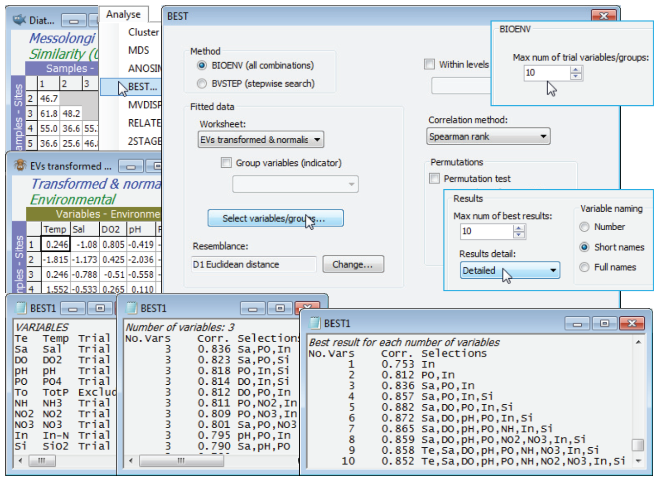
In fact, the match is even better with fewer abiotic variables. With the diatom resemblance matrix as the active sheet, run Analyse>BEST>(Method•BIOENV) & (Worksheet: EVs transformed & normalised), forcing exclusion of TotP under the Select variables/groups button, with the default of Euclidean resemblance and (Corr¬elation method•Spearman rank), and leaving the Permutation box un¬checked. On the Next > dialog, increase to (Max num of trial variables/groups: 10), since all 1023 combinations will run in a reasonable time. On the final dialog, (Results detail: Detailed) and (Variable naming•Short names). The results window and particularly the summary table of Best results for each number of variables shows that $\rho$ is maximised (at 0.88), for the 5 variables: Sal, DO$_2$, PO$_4$, In-N, SiO$_2$ and slowly decreases beyond that, as more variables are added. The best 3-variable solution (Sal, PO$_4$, In-N) does nearly as well ($\rho$ = 0.84), and on the principle of parsimony might be preferred as a simple ‘explanatory’ set of abiotic variables for these diatom communities. Causality, of course, is not established – see the comments in Chapters 11 and 12 in CiMC.


