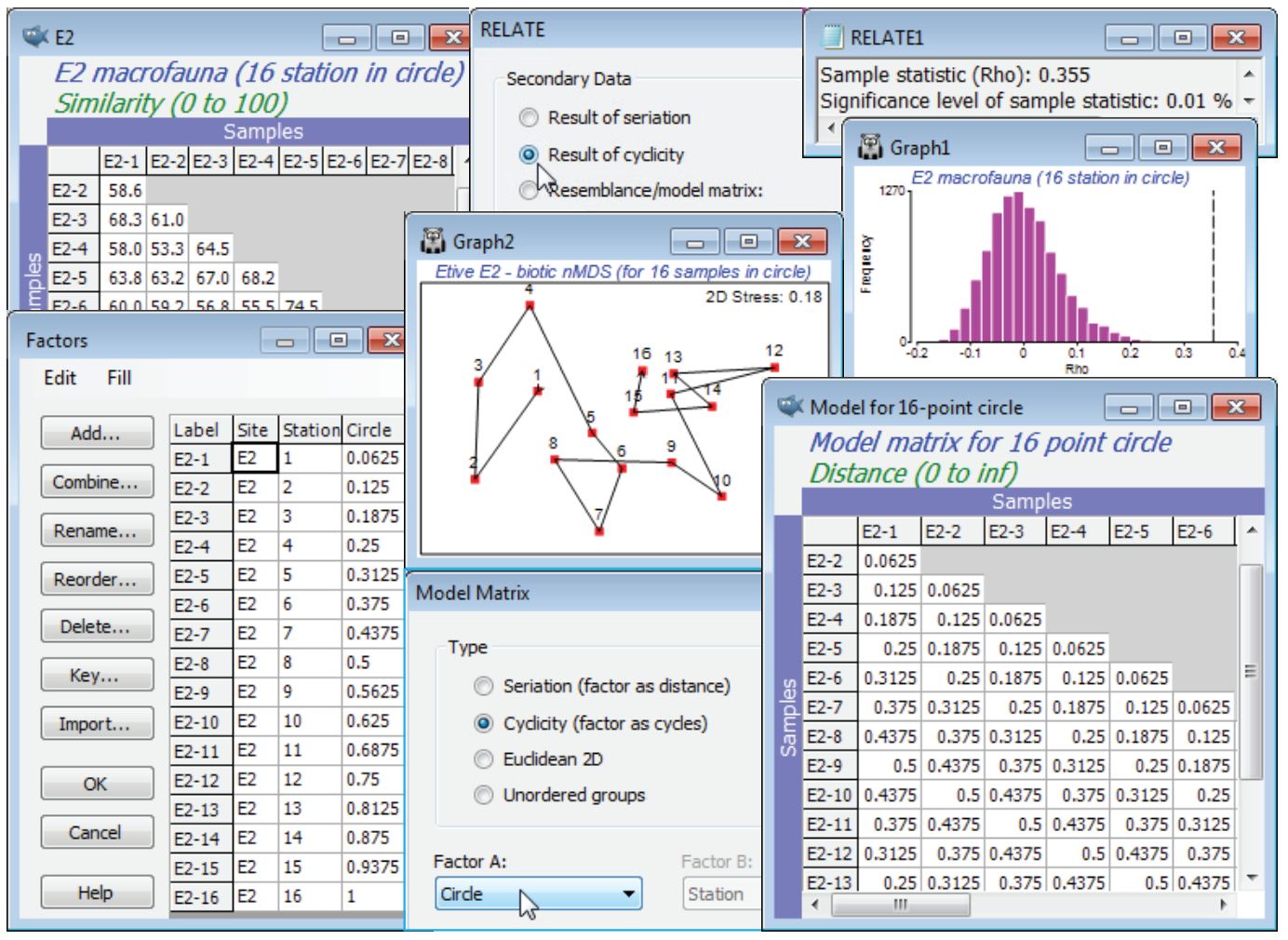
Model matrix for 2D Euclidean; Cyclicity (Sea-loch macrofauna)
The other two Model Matrix options are (Type•Cyclicity (factor as cycles)) and (Type•Euclidean 2D). The latter simply calculates, for example, distance between samples in a geographic layout when the x, y co-ordinates of the sample points are not held in a separate (environment-type) data sheet but as numeric factors in the biotic data. The corresponding model for sample locations in a 1D layout, given by a single factor, is just the (Type•Seriation) option, or equivalently, set up a Factor B with the same level (e.g. 1) for all samples and take the (Type•Euclidean 2D) option.
The (Type•Cyclicity (factor as cycles)) option in Model Matrix needs a numeric factor over the range (0, 1), representing the distances round a circle, where 0 and 1 are at the same point (or think of these as the angles at which those points are set, ranging over 0 to 1, not 0 to 360). The obvious examples of such data are in a time-series over a full seasonal cycle (see shortly), or a diel or tidal cycle, but we shall start with an unusual spatial example from studies described by Gage JD 1972 Mar Biol 14:281-297 (and analysed in a multivariate way by Somerfield PJ & Gage JD 2000 Mar Biol 136:1133-1145), of subtidal macrobenthos in Scottish sea-lochs. The subset of these samples used here is from three sites in Loch Etive, at each of which 16 samples (factor Stations, 1-16) were taken approx¬imately around the circumference of a 100m diameter circle at equal spacing. Over all three places (factor Site, E2, E6, E24) counts were made of a total of 186 species, in data file Etive macrofauna counts, directory C:\Examples v7\Sea-loch macrofauna. Open the data and select, for the moment, just the 16 samples from Site E2, by Select>Samples>(•Factor levels)>(Factor name: Site)>Levels>(Include: E2) & (Available: E6 & E24). On fourth-root transform and Bray-Curtis similarities, run the nMDS ordination and test the null hypothesis that there are no differences in communities at these 16 stations against the alternative of a circular structure (their spatial layout) with Analyse>RELATE>(Secondary data•Result of cyclicity). For simple cyclicity such as this, with equal spacing, no replication at each point, and an assumption that the stations are in correct order round the circle, the routine creates the model internally, and an explicit construction of the model matrix is not needed. However, it is instructive to create the model externally, from active sheet of the biotic similarities of the 16 samples, using Tools>Model Matrix>(Type•Cyclicity). The supplied (Factor A:) is not the Stations levels 1-16, but these numbers divided by 16, held in the factor Circle – in general the points, e.g. times, may not be equally spaced and the routine must be told how the start and end of the sequence relate to each other, hence the restriction to (0,1). The same RELATE test now results from using this cyclic model under (•Resemblance/model matrix: Model for 16-point circle), giving weak but still significant cyclicity ($\rho$= 0.355, p<0.01%).

