(Frierfjord macrofauna)

A data set not met elsewhere in this manual but which is used a great deal in CiMC, e.g. to start the description of 1-way ANOSIM permutation tests (Chapter 6), is from sub-tidal sampling by Day grabs for benthic macrofauna at 6 sites (labelled A-E, G) in Frier¬fjord/Langesundfjord, Norway. Four replicate grab samples were taken at each site, and the data matrix consists of counts of 110 macro¬benthic species over the 24 samples (Gray JS et al 1988 Mar Ecol Prog Ser 46: 151-165). The file is Frierfjord macrofauna counts(.pri) in C:\Examples v7\Frierfjord macrofauna – though an Excel version of the same data sheet Frierfjord macrofauna (Excel)(.xlsx) is also in that directory, as a reminder of the format necessary to read Excel sheets into PRIMER (Section 1).

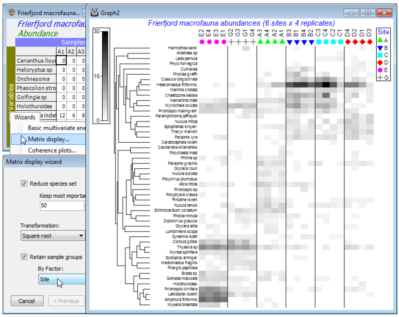
So, save and close any open workspace (e.g. Fal ws2), open Frierfjord macrofauna counts and with this as active sheet, run Wizards>Matrix display, taking the options (✓Reduce species set>Keep most important: 50) & (Transformation: Square root) & (✓Retain sample groups>By Factor: Site). The outcome needs one minor change, but for the moment look at the display and note that:

a) the species have been clustered, to place together species which tend to have similar patterns of abundance across the samples, and the dendrogram rotated to attempt to diagonalise the matrix;

b) the samples have been ordered also to diagonalise the matrix, which is arguably unhelpful here, so a later tidying-up step will replace the site alphabetic order, to reflect the spatial layout; but

c) the replicates are kept together within sites by the (✓Retain sample groups) instruction and the vertical bars divide the levels of the specified factor (the sites);

d) the abundance of each species in each sample can be gauged from the depth of shading, but this is on the requested square root scale, so the (rounded up) maximum value on the scale bar of 30 corresponds to a count of 900, and 15 to a count of 225, the same scale bar applying to all species – the number of values and maximum of the scale can be altered by the user;

e) the resulting plot makes it clear why the MDS and pairwise ANOSIM tests (Fig. 6.2 in CiMC) split the sites into three groups: E & G (in Frierfjord above the sill, where there may be seasonal anoxia), B, C & D (in Langesundfjord below the sill, where any pollutants from industrial inputs at the head of the fjord system will be well mixed) and A (the reference site in Oslofjord); and finally

f) distinctions can be seen between E and G on the basis of the replicates and with more subtlety between D and the group (B,C) – ANOSIM (Section 9) does not separate these latter two sites.

We now need to examine in more detail the decisions made and the routines employed to generate this Shade Plot, so that some limitations of the automated Matrix Display wizard can be relaxed. Note, however, that it is still often a good idea to produce an initial plot in this way, since many of the variations that are likely to be of interest can be achieved by one of the many options offered under the Graph>Special menu for shade plots, particularly the Reorder button.