Save sample/ variable order
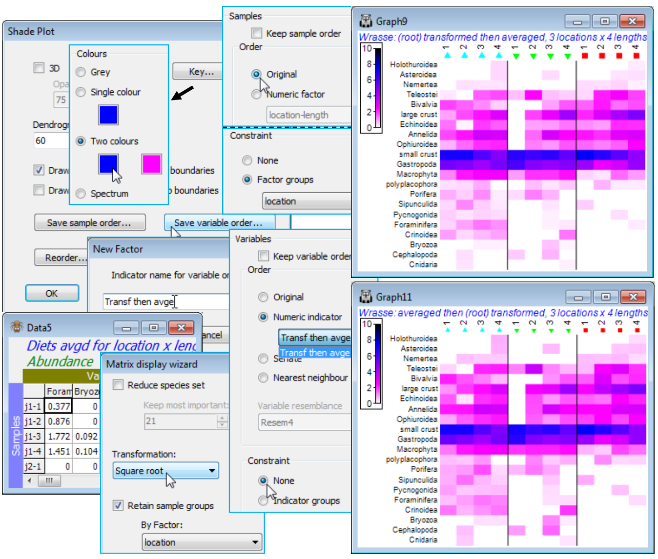
A final choice on the Special dialog for shade plots can be useful when planning to compare plots. Save sample order and Save variable order allow the current order (top to bottom for species and left to right for samples) to be saved to a factor or indicator respectively. These could be used to re-order the original matrix (with Edit>Sort>Rows or Columns) for a direct run of Plots>Shade Plot – i.e. without the reordering which is implicit in Matrix display – or they could be used as an entry to (Order•Numeric factor) or (Order•Numeric indicator) on the Reorder dialog. An example of the latter would be to compare the shade plots produced by trans¬forming then averaging (as performed above) with that obtained by first averaging, with Tools>Average>(Averages for factor: location-length) on the original Wrasse gut composition, then square root transforming the result in a run of Matrix display. Having run Special>Save variable order>(Indicator name for variable order: Transf then avge) on the first shade plot, under Special>Reorder on both plots take Variables> (Order•Numeric indicator Transf then avge) & (Constraint•None), and their species lists will align. The default plots from Matrix display are otherwise certain to have species in a different order, which will not make it easy to compare the two approaches. Note that a default run of Wizards>Matrix display under the (✓Retain sample groups>By factor: location) condition may also re-arrange the order in which the three locations are presented (since the attempted diagonalisation may differ). In general therefore, one could apply Special>Save sample order on the first array and Edit>Factors>Import this factor into the averaged matrix for the second array, thus ensuring that the two shade plots have both samples and species in the same order. In this straightforward case, however, it is simpler just to specify (Samples>Order•Original) under the Special>Reorder dialog for both plots, since we know that the matrix already has its samples listed in the required order (j1, j2, p2 locations, with length classes 1-4 within each, in that order). The comparison is given below, also demonstrating the other colour option not yet seen, mixing two colours between white and black. The conclusion is self-evident – the order in which averaging and a mild trans-formation (such as square root) are performed makes apparently negligible difference to the shade plot, and this is borne out in the multivariate ordination. In fact it is often observed to be the case that the various ways of displaying some form of meaned data do give very similar outcomes for balanced designs such as this – see the discussion in CiMC, Chapter 18. Save and close Wrasse ws.

