Matching variable sets; (Ekofisk oil-field study)
The final two sections of the Graph>Special dialog concern overlaying vectors and ‘bubbles’ of numeric values, rather than factors, either of the variables (e.g. species) from which the ordination has been created, or taken from an independent worksheet (e.g. of environmental variables) which contains the same sample labels as are found in the ordination. Note the matching principle: for all routines, the selected labels in the active sheet determine which samples are to be analysed, and any secondary data sheet supplied to that routine must include at least that sample label set, with names spelt in exactly the same way. The secondary data sheet can also contain other samples (which are ignored) and, of course, the required samples could be in a totally different order in the two sheets.
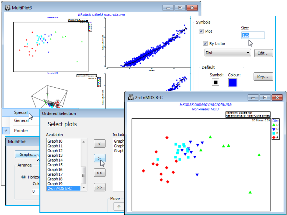
The superimposition of bubble plots and vectors on an ordination are illustrated for the benthic macrofauna assemblages sampled for 39 sites at different distances from the Ekofisk oilfield, in the Norwegian sector of the N Sea, sampled at one point in time, some years after operations began. This dataset was introduced at the beginning of the manual (Section 1) and the workspace Ekofisk ws last saved in Section 4. If this workspace is not available, open Ekofisk macrofauna counts and Ekofisk environmental from C:\Examples v7\Ekofisk macrofauna, square root transform the former (rename Square root) and compute Bray-Curtis similarities (B-C on sq rt). Run nMDS on this to obtain the 2-d ordination, 2-d nMDS B-C. (Note that renaming a graph removes it from the multi-plot – to return it, run Graph>Special>Graphs on the multi-plot and take its new name across to the Include list, moving it up to the head of the list in this case. Also, you may need to Rotate Data or Flip X or Y from the right-click menu to obtain the 2-d nMDS plot shown below). Already seen in the 2-d nMDS display are the four different symbols in the factor Dist, which puts the 39 sites into a priori defined groups depending on their distance from the centre of oil drilling activity – D: < 250m; C: 250m to 1km; B: 1km to 3.5km; A: > 3.5km. Use the Samp. labels & symbols tab to unclutter the plot by removing the labels and perhaps increase the symbol size, e.g. Size: 125.
The 2-d stress is quite low (0.09) and the ordination thus reliable (with the 3-d plot little improved, as seen in the Shepard diagram). There is a clear pattern of steady change in the community as the rig is approached (left to right). Note that sites within a few hundred metres of the rig (D), and thus close to each other, have quite variable assemblages, but distant sites (A), which can be 16km or more apart, are more tightly clustered – the opposite of expectation if the communities are not impacted by drilling mud disposal. The clear distinction between B and A (confirmed by ANOSIM, Section 9) is good evidence for an impact extending to more than 3 km from the oilfield centre.

