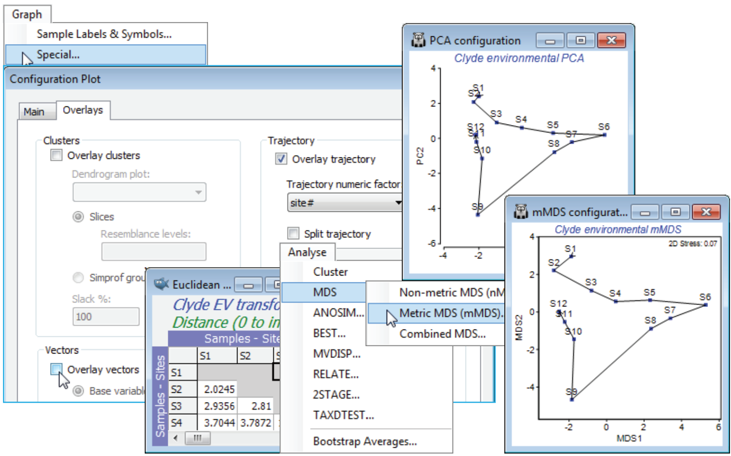
Trajectories on PCA

From the Graph>Special menu, remove the vector overlay by unchecking the (✓Overlay vectors) box on the Overlays tab, and on the same tab, join the points along the transect with (✓Overlay trajectory>Trajectory numeric factor: Site#) – if the factor doesn’t exist, create or import it, as seen under that Ranked variables heading. A better comparison would be of the current PCA with mMDS not on the ranked variables but on the same Euclidean distances as created from normalised and transformed variables here, so you may wish to run that Analyse>MDS>Metric MDS (mMDS) routine. This indicates one rather obvious difference: mMDS works from the resemblance matrix and PCA from the data matrix underlying that. A more important distinction is that mMDS does not project the points from the high-d to low-d space as in a PCA, but more carefully arranges them in order optimally to match the low-d Euclidean distance structure to the original distance matrix. Here however, all these ordination cases are effectively indistinguishable: the samples largely lie on a 2-d plane in the 11-d space making it easy for both methods to display an accurate 2-d picture.

More interesting is the fact that the PCA (or mMDS) of the abiotic variables is an excellent match to the nMDS of the assemblage (also in Section 11), whether based on biomass, abundance or both, and this observation motivates the BEST routine of Section 13. (Note that a PCA of the biota is poor by comparison, since it implicitly uses Euclidean distance rather than an assemblage-based coefficient such as Bray-Curtis – and it actually fails to display a convincing species gradient even though there patently is one there. Choice of a relevant similarity is much the most crucial decision to make in multivariate analysis – a point seen again in Section 14.)