Basic MVA for a priori unstructured biotic data
In the Fal estuary study, where there are environmental data matching each of the 27 sites, it is not unreasonable to consider a different form of analysis, in which creek designations are considered secondary to the biotic relationships among sites in relation to the differences in the heavy metal concentrations (and such an analysis, by LINKTREE, is seen for this data in Chapter 11 of CiMC). In other words, we can choose to ignore the Creek factor and analyse the 27 sites as unstructured. Another obvious example of this type of data, which we saw extensively in Section 6, is the zoo-plankton study of 57 sites in the Bristol Channel and Severn Estuary, which are laid out in a grid, and the primary analyses concern both a clustering of those sites into data-determined groups, and observation also (Section 8) of a more continuous gradation in the MDS plot – relating to salinity.
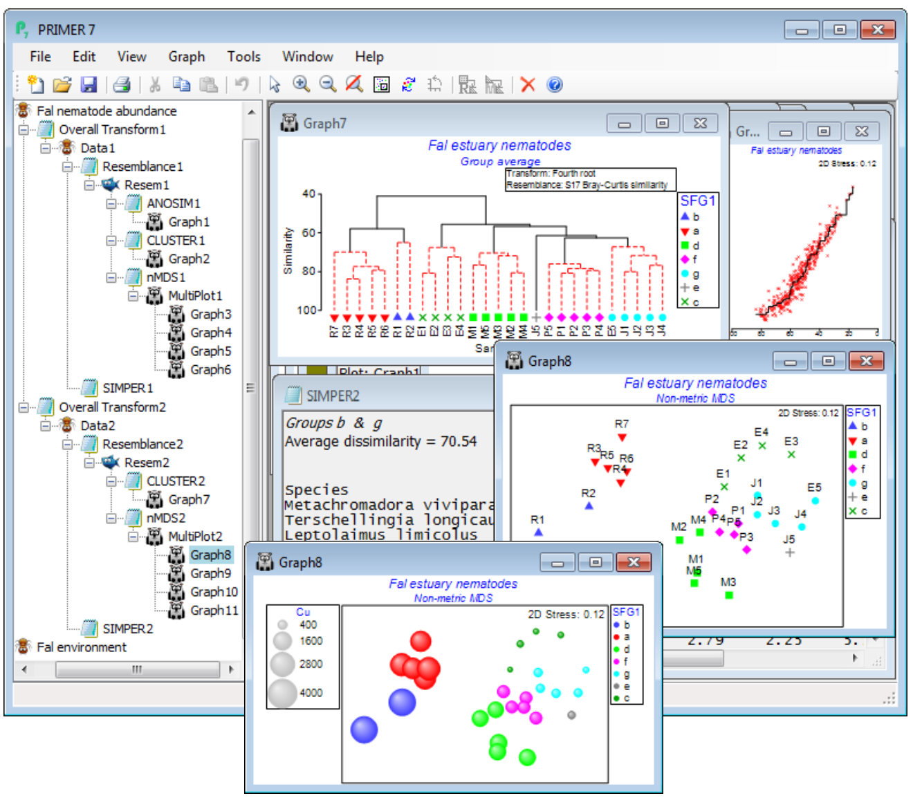
Rather than re-open the Bristol Channel data again, we run through Wizards>Basic multivariate analysis once more on Fal nematode abundancens but this time unchecking the (✓ANOSIM) box – the (✓SIMPROF) box is automatically now ticked. The output sequence in the Explorer tree looks similar (without the ANOSIM results of course) but now the dendrogram indicates the clusters of sites which are significantly separated by the series of SIMPROF tests (Section 6) – red dotted lines indicating sub-clustering which has no statistical support, with interpretable structure identified by black continuous lines. In fact, this largely accords with the creek designations – which was partly to be expected given the large pairwise R values in the previous ANOSIM test, but further division of the assemblages within creeks is more or less confined to two outlying sites in Restronguet. The SIMPROF test has automatically created a new factor, SFG1, of its 7 identified groups (one is the singleton J5) and this is available to all sheets and plots on this branch – and on the previous branch actually, since it back-propagates up to the Fal nematode abundance sheet and then forwards down the first branch – and SFG1 is displayed as symbols on the nMDS plot. In order to strengthen the visual association with the clustering, on the dendrogram (Graph7) you may wish to take Graph> Sample Labels & Symbols>Symbols(✓Plot)>(✓By factor SFG1). The SIMPER output is now in terms of these 7 SFG1 groups, rather than the previous Creek designations, naturally. It would also make good sense to superimpose individual heavy metal concentrations (or other abiotic variables) on the nMDS ordination, in a bubble plot. So, open Fal environment from the same directory, and with Graph8 as the active window, right-click over this (or Graph) and Special>Main>(Bubble ✓Bubble plot)>(Worksheet: Fal environment) & (Variables: Cu) – you will need to take Change to select this variable, or you might prefer to Include multiple variables, for a segmented bubble plot. For a single variable, you might prefer the look of (✓3D effect) and, back on the Graph>Sample Labels & Symbols menu, uncheck the (Labels✓Plot) box and also (✓Plot history) on General.

