(Morlaix macrofauna, Amoco-Cadiz oil spill)
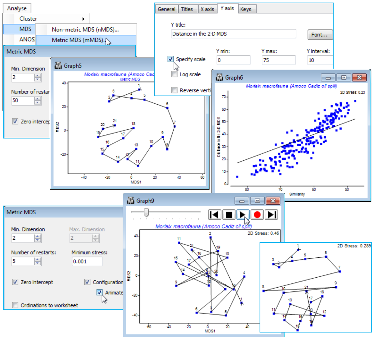
Close the World cities worksheet (it will not be needed again) and re-open workspace Morlaix ws, from earlier in this section. It contains the data sheet Morlaix macrofauna abundance, fourth-root transformed and with Bray-Curtis similarity matrix, Resem1, on which to carry out 2-d mMDS, with Analyse>MDS>Metric MDS (mMDS), taking all the default options, and making the time factor the labels rather than the symbols, on Samp. labels & symbols – you should also join the points in time order as previously demonstrated, with Special>Overlays>Trajectory. The below also adjusts the scales of the Shepard plot by clicking on them (X axis & Y axis tabs). You might also enjoy repeating this 2-d MDS with, say, (Number of restarts: 5) & (Minimum stress: 0.001) and (Animate) switched on. Make sure that you make the above symbol and label changes, and especially the trajectory overlay, before starting the animation, with ![]() . Even with the rather small number of points here (21) and the clear pattern, note how often the convergence does get trapped in a sub-optimal solution. This is also clear from the results window, mMDS1, from the initial run with 50 restarts, with only 20-30% of those converging to the (probably) lowest stress of 0.235.
. Even with the rather small number of points here (21) and the clear pattern, note how often the convergence does get trapped in a sub-optimal solution. This is also clear from the results window, mMDS1, from the initial run with 50 restarts, with only 20-30% of those converging to the (probably) lowest stress of 0.235.
Marginally higher stress is to be expected from an mMDS solution than an nMDS one, even if the Shepard diagram does show a linear fit through the origin to be an excellent description of the relationship of dissimilarities to plot distances – this is because nMDS’s monotonic regression can make fine-scale steps to ‘chase’ the data even when displaying essentially a straight line (especially if there are few samples and therefore not too many points on the Shepard plot to ‘chase’). But a high stress of 0.24 for mMDS, compared with a low one of 0.09 for nMDS, shows a drastically poorer fit for the former, and the reason is clear from the Shepard diagram: the points do form a fairly tight relationship with relatively low scatter (i.e. will fit well into a 2-d representation) but this is not linear through the origin, the assumption for metric MDS. In fact, the mMDS routine appears to be telling us that it can make good sense of these dissimilarities as a 2-d configuration, provided it ignores the model we have specified! It is the lack of fit to the model, rather than innate distortion in the 2-d solution (i.e. high variability in distance at each dissimilarity value), which is largely inflating the stress – this is also seen in the way the mMDS is similar to the earlier nMDS.

