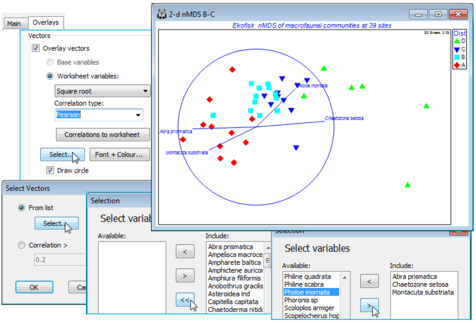
Vector plots for species

One tempting alternative, commonly found in the literature, is to plot (species) variables as vectors on the MDS plot (see below). They are directional lines emanating from a common origin, pointing in the directions in which those species numbers increase, and of length reflecting the strength of pattern in those species counts along that direction. Such a vector plot can have its origin anywhere (there is a common misconception that its placement or overall size matters) and PRIMER chooses to locate it the left side of the plot – deliberately non-central to make the point about arbitrariness of its origin. The perceived advantage of a vector plot is that it can display the relationship of many species to the ordination configuration in a single plot. But, in reality, it rarely succeeds. Firstly, a vector assumes the relationship is strictly linear, but the above bubble plots for Abra prismatica and Montacuta substriata show threshold relationships, present at consistent numbers until a (different) point is reached, closer to the oilfield, when numbers drop to zero. Even worse is Pholoe inornata whose relationship to the gradient is not even monotonic, because it is an opportunist increasing in numbers closer to the impact but decreasing again when the impact becomes strong, within 100m. Of the above four bubble plots, only Chaetozone setosa would be well described by a linear fit of (root) counts to (x,y) co-ordinates of the MDS plot. Secondly, vector length measures (Pearson) correlation of transformed counts to these axes (see Chapter 7 of CiMC), not just a purely linear construction but also one that ignores the universal scaling of the bubble plots – if a species has very low numbers throughout and thus could not contribute much to the similarities and ordination, it might still have a large vector if its numbers gently decrease (or increase) closer to the oilfield. In other words, vector plots only make sense in the bubble plot context above, of judging relative contributions to the ordination, where species have been standardised prior to analysis, i.e. where species are given the same weight in similarity calculations, irrespective of their overall abundance. These are compelling reasons for never using a vector plot of species! Nonetheless, a vector plot can be implemented as follows. On the MDS graph 2-d nMDS B-C, under Graph>Special turn off (✓Bubble plot) on the Main tab, and on Overlays take (Vectors✓Overlay vectors)>(•Worksheet variables: Square root)&(Correlation type: Pearson)&(✓Draw circle)&(Select>•From list>Select), and leave only species Abra prismatica, Chaetozone setosa, Montacuta substriata and Pholoe inornata in the Include box. The circle indicates a (multiple) correlation of 1 of that species to the 2-d MDS x, y co-ordinates (see the ‘Vector plots’ heading in Chapter 7 of CiMC for discussion of this and the alternative(s) to Pearson correlation). Clearly, the resulting vector plot carries limited information compared with bubble plots: the different threshold responses of Abra prismatica and Montacuta substriata cannot be captured, likewise the non-monotonic relation for Pholoe inornata.