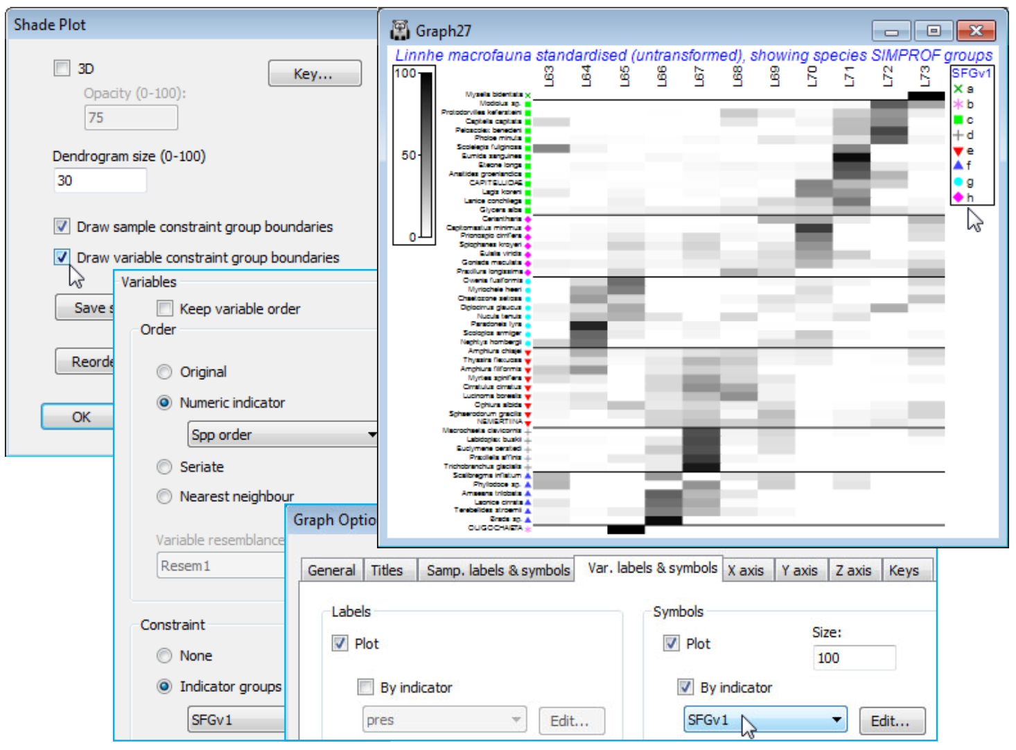
Shade plots showing coherent sets & variable boundaries

In order to display a shade plot carrying precisely the same information as the coherent species line plots, first save the species order in the above shade plot – in order to make it easier to compare the two shade plots – using Graph>Special>Save variable order>(Indicator name for variable order Spp order), then with the active matrix this time as the species-standardised (but not transformed) sheet Data2, run Plots>Shade Plot and note that now many species rows contain the darker entries, i.e. those whose dominant abundances are in a single year, the common scale (0, 100%) now being relative to the total abundance for each species over all years. Rearrange the species in the previous order by Graph>Special>Reorder>Variables>(Order•Numeric indicator Spp order)&(Constraint• Indicator groups SFGv1), and after OK returns you to the first of the Special dialog boxes, take (✓Draw variable constraint group boundaries). This is the first time we have seen horizontal lines on the shade plot, separating the coherent species groups, and it certainly helps the visual message. The plot below also adds symbols for the species groups, using the Var. Labels & Symbols tab as previously, since the key does make a link to the earlier line plots of these groups, for which the indicator level (lower case letter) is given in the sub-titles. Remember also that you can re-order the constituents of a key by clicking on the key and using the Move arrows, which has been done here to re-arrange the indicator levels alphabetically. Abbreviations of the species names can sometimes be necessary and this is simply achieved on the Var. Labels & Symbols tab again, by putting them into another indicator Spp abbrev and (Labels✓Plot>✓By indicator Spp abbrev).