Interpreting PCA vs MDS pairwise plots

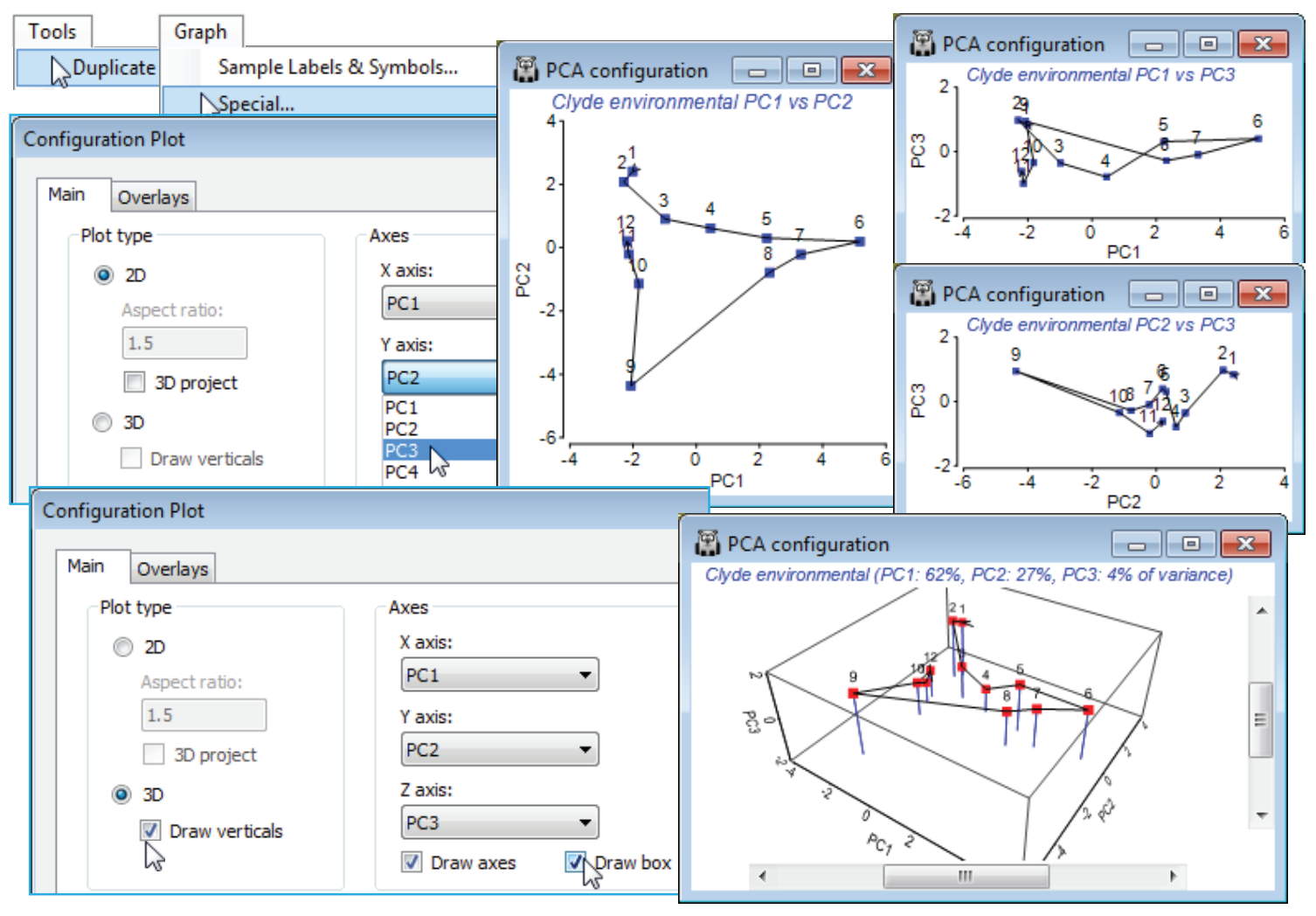
Another subtle distinction from MDS is that only a single PCA graph window is produced initially, allowing a choice between displaying a 2-d or 3-d scatter plot. This is because the PC algorithm generates just one solution, with as many PCs as requested: a 2-d PCA is just the first two axes of the 3-d PCA, etc. With MDS, the 2-d and 3-d plots are entirely separate solutions and thus held in different windows. It is possible, starting from a 3-d MDS window, to take Graph>Special>Main>(Plot type•2D) and generate the three pairwise plots: (MDS1,MDS2), (MDS1,MDS3), (MDS2, MDS3) – as remarked above, this gives an alternative static view of the 3-d solution, rather than an arbitrarily projected view of the 3-d box. But, unlike PCA, do not expect the (MDS1, MDS2) plot from this to be exactly the same as the purely 2-d MDS solution! They mean different things and the purely 2-d MDS solution will always be the better representation of the original relationships.

It is clear from the Clyde environmental 3-d PCA below that a 2-d ordination is perfectly adequate (noted previously from the % variance explained). The various 2-d and 3-d plots show how little absolute variation there is on the third axis – another good reason for preserving the aspect ratio, as PRIMER does for all ordinations, i.e. a distance of 0 to 2 units is the same on all axes. You may even need to change the default scaling, (✓Specify scale) on the Z axis tab, to (-2, 2) to get the plot below, to avoid too much compression of the PC3 axis! Save and close the Clyde ws workspace.