Basic MVA for structured data (Fal nematodes)

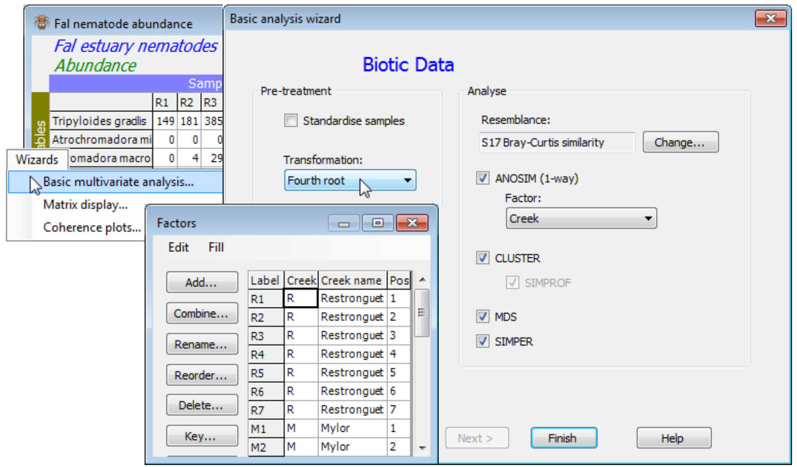
The benthic faunal study in the Fal estuary, Cornwall UK, was seen in Section 4. Sediment samples were taken at a total of 27 sites across 5 creeks running into the Fal estuary, with differing levels of heavy metal contamination from historic tin and copper mining – 7 sites in Restronguet (R) and 5 in each of Mylor (M), Pill (P), St Just (J) and Percuil (E) creeks. The existing workspace, Fal ws, concerns only the meiofaunal copepod community, and in Section 17 we shall see the macro¬faunal component, but open here the nematode assemblages, Fal nematode abundance from C:\Examples v7\Fal benthic fauna, into a clear workspace (Fal ws2). Wizards>Basic multi¬variate analysis then offers the sequence of analyses shown below – in particular the routine picks up the existence of a Creek factor with repeated levels and checks the ANOSIM not SIMPROF boxes. In this case, a more severe transform is desirable to downweight the highly abundant Metachromadora vivipara, so change to (Transformation: Fourth root) – a shade plot (see later, and Section 4) helps here.

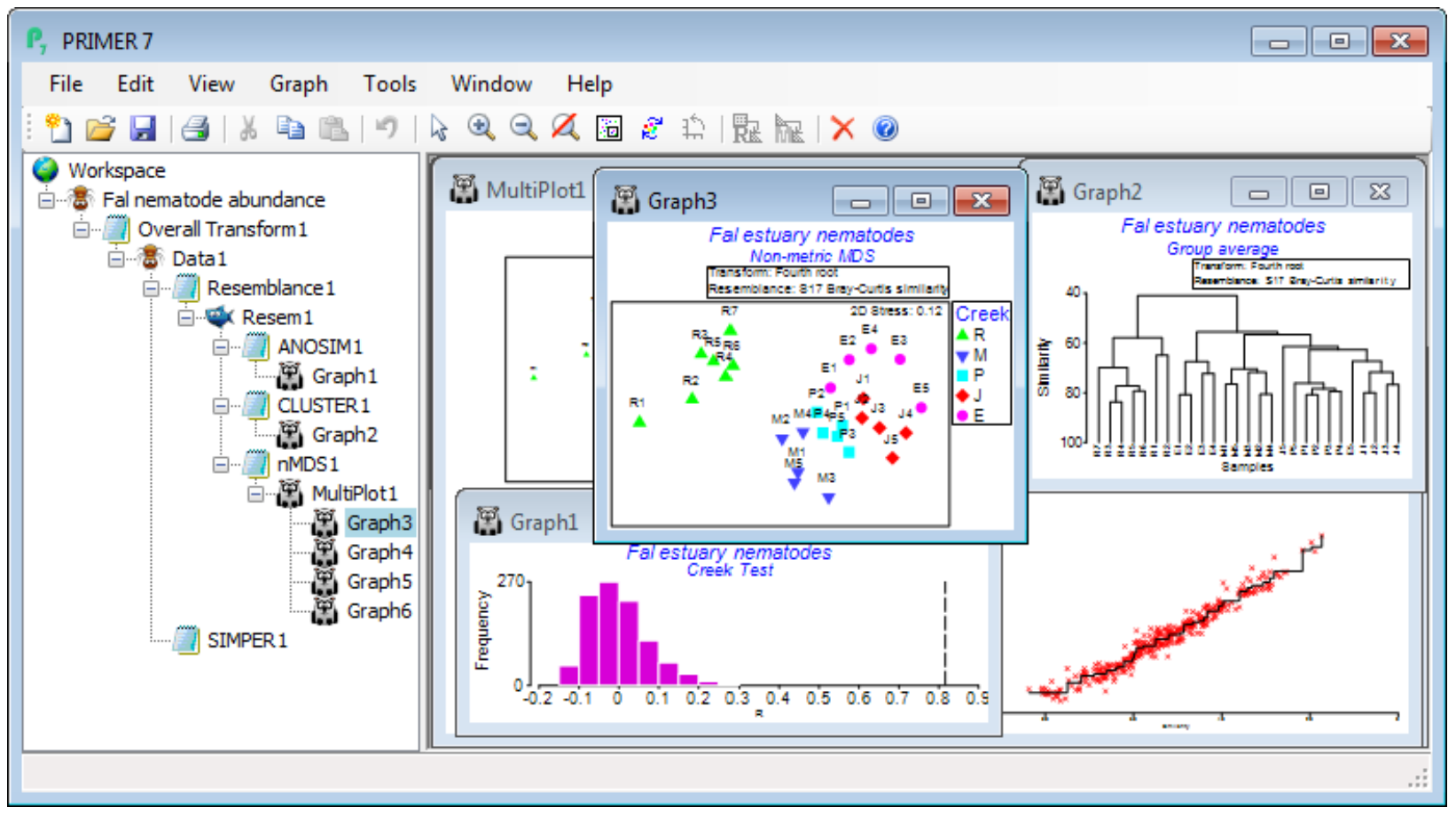
The main intention of the Wizards is to aid understanding of the steps involved, by examining the sequence of windows created in the Explorer tree. In this case, you can create precisely the same outcome by running the following. On Fal nematode abundance, take Pre-treatment>Transform (overall)>(Transformation: Fourth root) and, on the resulting transformed sheet Data1, Analyse> Resemblance>(Measure•Bray-Curtis similarity) & (Analyse between•Samples), giving Resem1. On Resem1, Analyse>ANOSIM>(Model:One-Way - A) & (Factors A: Creek)>(Type: Unordered) leads to ANOSIM test results, testing for significance of differences among creeks overall and pair-wise, in ANOSIM1, and a histogram of the null distribution for the overall (global) test, Graph1. On Resem1, Analyse>Cluster>CLUSTER>(Cluster mode•Group Average)&(✓Plot dendrogram) but without the SIMPROF box ticked, displays a standard UPGMA clustering in Graph2. Again on Resem1, Analyse>MDS>Non-metric MDS (nMDS), with the defaults of (Min. Dimension: 2) & (Max. Dimension: 3)&(Number of restarts: 50)&(Minimum stress: 0.01)&(Kruskal fit scheme•1)& (✓Configuration plot) & (✓Shepard diagrams), gives the results window for MDS, nMDS1, which contains important information on how many times the lowest stress solution was observed in the 50 random restarts (if only a handful of times, consider running again with more restarts), and then the Multiplot1 window, which contains the (best) 2-d and 3-d ordination plots, along with Shepard diagrams. Clicking on any of these plots (or the + sign in front of the Multiplot1 icon) unrolls the four individual plots in the Explorer tree, Graph3 to Graph6. Finally, on the data sheet Data1, not the resemblance sheet Resem1 note, taking Analyse>SIMPER>(Design•One way) & (Factor A: Creek) & (Measure•Bray-Curtis similarity), with the other two boxes ticked, will give the detailed results window SIMPER1, breaking down the average dissimilarity between pairs of the ANOSIM groups (the creeks) into contributions from each species – see later this section.

The main conclusions here are that there are clearly significant differences overall between creeks (global R very large at 0.816, p<0.1%) and, almost equally clearly, between all pairs of creeks – the only pairwise R value which drops as low as 0.5 is between St Just (J) and Percuil (E) (p<2.4%). Other pairwise R values are in the range 0.75-0.99, and all of them are the largest obtainable values – greatest separation possible – in all permutations of the labels between the pair of creeks (i.e. 126 permutations for two creeks which both have 5 replicates, and 792 if Restronguet’s 7 replicates are involved). In keeping with the pairwise ANOSIM R values for Restronguet (all R>0.9 even though the variability in Restronguet sites is large), the nMDS plot displays the very different nematode assemblages for that creek – it has by far the highest sediment concentrations of heavy metals.