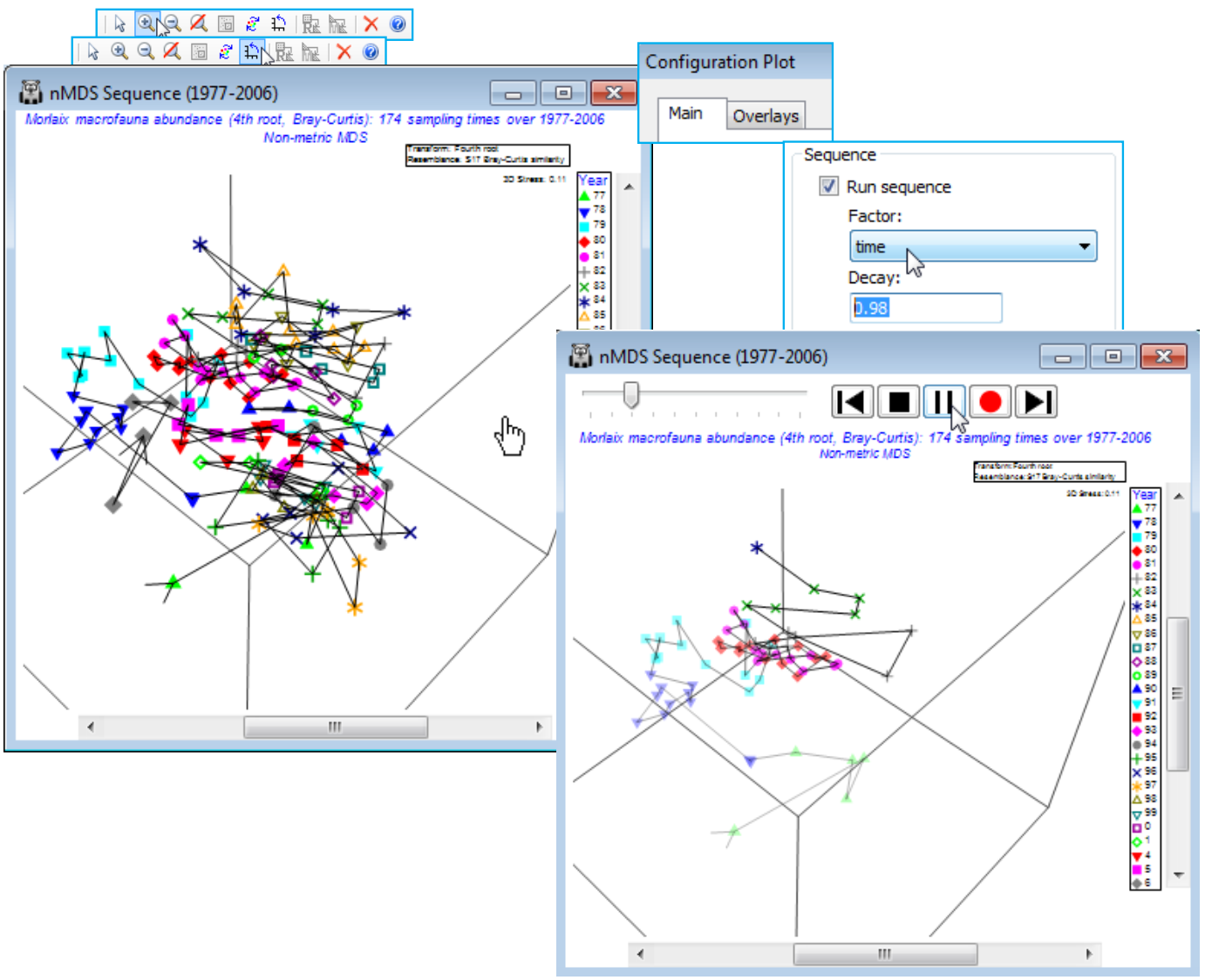
Sequence animation, captured in 2- & 3-d
The time pattern above is evident from simple addition of the trajectory but there are occasions when a confused MDS plot results from a longer sequence of points, especially if the multivariate structure tracks back on itself, repeating earlier states. Viewing the 3-d MDS is often helpful, and a trajectory can be added there, in exactly the same way. However, it can also help to elucidate the sequential pattern dynamically. PRIMER 7 has thus added sequence animation as a further option for 2- or 3-d ordination plots. This adds the samples to the ordination plot in sequential (e.g. time-ordered) fashion, including the joining lines of the trajectory if that is selected (as it usually would be). The earlier points and lines in the sequence gradually fade out as the later ones are plotted, allowing a more uncluttered view of progression of the multivariate structure. This is accessed by Graph>Special>Main>(Sequence✓Run sequence), supplying the numeric factor which gives the temporal (or other sequence) order and specifying a Decay parameter (in the range 0 to 1), which controls how quickly the earlier parts of the sequence fade. The default of 0.9 corresponds to a rather slow fade so that most of the earlier points from a short sequence remain visible throughout. Other contexts may need an even slower (0.98) or faster (0.5) decay, both these being used below.
The sequence animation can be run with or without capturing the dynamic display in digital movie form. From the Main tab, on entering the ordering factor and decay, and pressing OK, the standard video controls are displayed, and these operate just as described two pages ago (for Graph>Spin on a 3-d MDS plot): ![]() to start or pause,
to start or pause, ![]() to stop, with the slider varying the animation speed. A further option available here is to take one sequence step forwards or backwards with
to stop, with the slider varying the animation speed. A further option available here is to take one sequence step forwards or backwards with ![]() or
or ![]() . If
. If ![]() has initially been pressed, recording starts with
has initially been pressed, recording starts with ![]() and REC appears; stop by
and REC appears; stop by ![]() . If correct entries have already been set in a previous run, repeats need only a selection of Graph>Sequence.
. If correct entries have already been set in a previous run, repeats need only a selection of Graph>Sequence.
To demonstrate this sequence animation, File>Open the plot file nMDS Sequence (1977-2006).ppl into the current Morlaix workspace. This is a PRIMER binary-format file of a 3-d MDS plot for a much longer run of years of grab sampling for benthic macrofauna at station Pierre Noire in the Bay of Morlaix, see Dauvin and Thiébaut references above. The data matrix is not accessible from this file – it is used here only as a dynamic demonstration of the (static) MDS plot in the Thiébaut et al analysis – but it is worth noting that a PRIMER *.ppl file does carry around with it enough of the background information on the samples (the factor sheet) to allow the ordination configuration to be annotated in different ways, rotated etc. So this could be a flexible format for distributing plot results to others (who have access to PRIMER 7) but where the data itself cannot be released.
Take Zoom In (and centre with the scroll bars) and manually Rotate Axes, but the pattern is still a little confused. Does the benthic community approach its 1977 pre-oil impact state (if that one year is representative of this!), or are more regional or global-scale processes of environmental change at work? A slightly clearer demonstration of the time course is produced by Graph>Special>Main >(Sequence✓Run sequence)>(Factor: time)&(Decay: 0.98) and ![]() . You will find that rotating the plot while the sequence unfolds is of some help, and perhaps varying the speed with the slider. The plot captures not just the inter-annual trends but also (if carefully watched) the scale of the seasonal cycle in relation to those trends (there is an average of nearly 6 sampling times across each year).
. You will find that rotating the plot while the sequence unfolds is of some help, and perhaps varying the speed with the slider. The plot captures not just the inter-annual trends but also (if carefully watched) the scale of the seasonal cycle in relation to those trends (there is an average of nearly 6 sampling times across each year).

