(Biomarkers for N Sea flounder)

The directory C:\Examples v7\N Sea biomarkers holds a data sheet N Sea flounder biomarkers(.pri) of biochemical and histological biomarkers measured concurrently on flounder caught at 5 North Sea sites (labelled S3, S5, S6, S7 and S9), running on a putative contaminant gradient from the mouth of the Elbe (S3) to the Dogger Bank (S9). It is a multivariate study because all variables were measured on each of 50 (pools of) fish, consisting of 10 sample pools from each site. This was part of a larger practical workshop on assessing ‘biological effects’ techniques for detecting pollution in the marine environment – the IOC Bremerhaven workshop (Stebbing ARD, Dethlefsen V, Carr M (eds) 1992, Mar Ecol Prog Ser 91, special issue). The 11 biochemical and sub-cellular variables measured: EROD, lysosomal acridine orange (LYS AO), lysosomal neutral-red retention (LYS NRR), pinocytosis (PINOCYT), oxyradicals (OXYRAD), endoplasmic reticulum (END RET), N-ras, ubiquitin, cathepsin D (CATH D), tubulin and lipid vacuoles (LIPID VAC), which are a mixture of continuous, heavily discretised and (one) presence/absence variables.

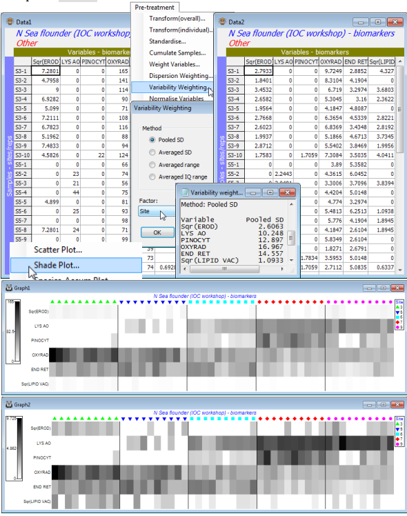
Open the N Sea flounder biomarkers sheet; note this time the 11 variables are columns and the 50 samples the rows, with a defined Site factor. Highlight, then select, only the 6 continuous variables EROD, LYS AO, PINOCYT, OXYRAD, END RET and LIPID VAC. They are all statistically well-behaved variables without strong outliers though the replicates for EROD and LIPID VAC are somewhat right-skewed, so it might be beneficial to highlight these two and take Pre-treatment> Transform(Individual)>(Expression:Sqr(V)) for a mild square root transform of those variables. *Pre-treatment>Variability Weighting>(•Pooled SD) & (Factor:Site) then results in a sheet in which the columns (variables) are just divided by the pooled SD values given in the results window ( Variability weighting1). The Data2 sheet is now ready to go into the Analyse>Resemblance> (Measure•Euclidean distance) routine of the next section. (Note that, though the Pooled SD divisor is really designed for continuous data, nothing goes dramatically wrong by leaving all 11 variables in the computations, though the discrete variables need to be at least ordered categories, as here).

Finally, the effect on the relative contributions of each of the 6 variables to the Resemblance calculations, before and after the Variability Weighting, can be neatly seen by submitting both Data1 and Data2 to Plots>Shade Plot. The (transformed) EROD and Lipid variables would clearly be largely ignored without the rescaling but, less trivially, the variable clearly given greater weight (darker shading) by the rescaling is LYS AO, seen to have consistently high or consistently low values for replicates from the same site, in the original plot. The plots have been slightly modified, simply to accentuate the site differences on the x axis, using the extensive menu choices, e.g. for labels and adding symbols, Graph>Sample Labels & Symbols>(Symbols:(✓Plot) & (✓By factor) & Site) and taking off the tick box for Labels. This is a generic menu that covers many types of plot and will be seen again in Section 6 and beyond. Also, there are Special menus applying only to individual types of plot and one of those is demonstrated by the dividing lines between sites, which are produced by Graph>Special>Reorder>(Samples:Constraint•Factor groups:Site). The many other options on this Special menu for the shade plot routine are discussed in Section 10. Save the workspace as N Sea ws.