Quantitative measures on P/A data; Unravelling resemblances; Scatter plots
It is instructive to draw the other links between quantitative coefficients and the presence/absence measures they reduce to, when calculating them on a P/A matrix. Pure distance measures such as $D_1$, $D_6$, $D_7$ and $D_{10}$, which are not averaged in some way over the number of species, clearly cannot reduce to the dimensionless ratios in the P/A similarity definitions above. Similarly, $D_{15}$, $D_{16}$, $S_{15}$ and $S_{19}$ are not of interest in this context because they are not just functions of $a$, $b$, $c$, $d$ for the two samples but bring in species for all other samples, in their species standardisations. However, the other quantitative measures mainly reduce to simple monotonic functions of four P/A similarities: $S_1$ (simple matching), $S_7$ (Jaccard), $S_8$ (Sørensen) and $S_{14}$ (Ochiai P/A). Of course, as defined, the relationships will be between $D$ and $(1 – S/100)$. To be precise: $D_2$ reduces to the square root of the complement of $S_1/100$; both $D_3$ and $D_{17}$ go to the square root of $2(1 – S_{14}/100)$, $D_4$ to $\cos^{-1} (S_{14}/100)$ and $S^{Och}$ to $S_{14}$; $D_8$ reduces to the complement of $S_7$, $D_{11}$ to the square root of that complement, and $S^{Can}$ to $S_7$. As noted earlier, $S_{17}$ reduces to $S_8$ and, finally, $S_{18}$ goes to $S_{13}$.
In less technical description: average Euclidean distance (squared) is the natural counterpart of simple matching (they are both functions of the number of joint absences); chord, geodesic and Hellinger distance, and naturally quantitative Ochiai, all have an affinity to the P/A form of Ochiai; Czekanowski’s mean character difference, the divergence coefficient and Canberra similarity all relate to Jaccard; Bray-Curtis reduces to Sørensen and, unsurprisingly, the quantitative and P/A forms of the Kulczynski coefficient converge, e.g. as strong transforms force the data towards P/A.
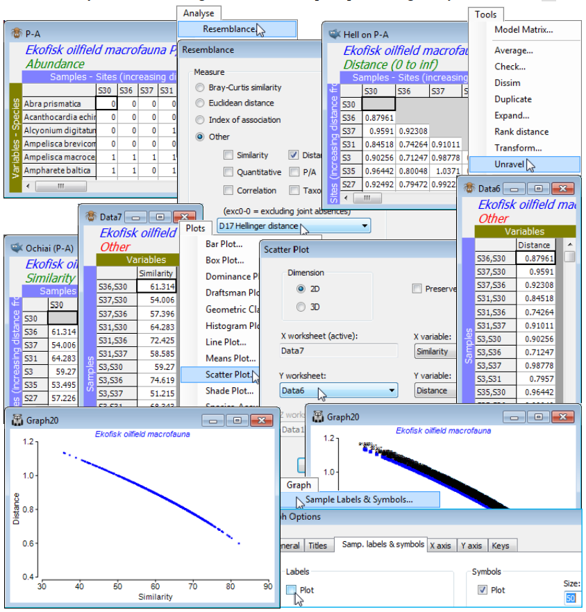
Demonstrate one of these points for the Ekofisk abundance data in the Ekofisk ws – which should still be open – by calculating Hellinger distance ($D_{17}$) on the presence/absence data produced from the macrofauna sheet, and comparing this with the Ochiai P/A coefficient ($S_{14}$). Thus:
a) With Ekofisk macrofauna counts as the active window, Pre-treatment>Transform(overall)> (Transformation: Presence/absence) to produce the P/A matrix, then renamed P-A (forward slash is not a permitted symbol in the Explorer tree, since these may sometimes be filenames);
b) On P-A, Analyse>Resemblance>(Measure•Other: D17 Hellinger distance) & (Analyse between •Samples), renaming the Resem sheet to Hell on P-A. [Do not take ‘Add dummy variable’ here – or routinely (always think carefully about it first!). It will have negligible effect here on relative distances because there are no denuded samples at all. However, the option is permitted with all measures and could make sense, in the presence of blank or near-blank samples (which are then required to have zero or near-zero distances/dissimilarities), for all those coefficients identified above (as ratios). This is essentially anything with a $y$ term or $p_{12}$ in the denominator, since these give an Undefined! resemblance entry for blank samples. The pure distance measures $D_1$, $D_6$, $D_7$ and $D_{10}$ will be unchanged with an added dummy, as will the species-standardised $S_{15}$ (which promptly has to remove the just-added dummy variable since its range $R_i$ over samples is zero!)]
c) On Ekofisk macrofauna counts take Analyse>Resemblance>(Measure•Other:S14 Ochiai(P/A)), renaming the result to Ochiai (P/A).
To view the relationship between these matrices, exploit two of the new features in PRIMER 7:
d) Run Tools>Unravel on both Hell on P-A and Ochiai (P/A), to turn these triangular matrices into long single columns (unravelling the rows), possibly now called Data6 and Data7.
e) With Data7 (say) as the active sheet, take Plots>Scatter Plot>(Dimension•2D) & (X variable: Similarity) & (Y worksheet: Data6) & (Y variable: Distance) – of course the X worksheet is the active Data7 – to see that Hellinger distance (on P/A data) is a decreasing function (near-linear here) of Ochiai similarity. The unnecessary sample labels can be removed by Graph>Sample Labels & Symbols, unchecking Labels✓Plot, and perhaps reducing the Symbols to Size: 50.

