3-way crossed /nested design (Tees Bay macrofauna)
The two other possible 3-way designs can be written C(A$\times$B) and B$\times$C(A). The first is straight-forward: an example might be of locations (A) each containing the same set of habitat types (B), and within each combination of habitat and location a number of sites (C) are randomly chosen, with replicates taken at each site. The ANOSIM tests are again effectively 2-way cases, with A and B flattened by combining them into a single factor (AB), so the design for testing C is the nested case C(AB), and the tests for A and B using the crossed 2-way A$\times$B design, with the levels of C as ‘replicates’ (averaging over the original replicates is, as usual, on the rank similarities). The 3-way C(A$\times$B) choice handles all this automatically, naturally, and again factors can be ordered or not.
The remaining possibility B$\times$C(A), in which B is crossed with all levels of C, the latter nested in A, is more complex and for some tests requires variations of the 2-way test statistics (fundamentally still either average R, R$^\text{O}$ or $\rho$ constructions, however) and a modified permutation procedure in which whole sets of sample labels are permuted together. This is discussed extensively in CiMC, towards the end of Chapter 6 and in Table 6.4, and will not therefore all be repeated here. We will just use the same example as in CiMC to illustrate setting up and interpreting these tests. This is the Tees Bay macrofauna data introduced in Section 8 as an example of time-series trajectories in ordinations (see also Fig. 6.17 in CiMC), with workspace Tees ws and data Tees macrobenthic abundance in C:\Examples v7\Tees macrobenthos. Factors are Area (A), Year (B) and Site (C), with the 4 areas of Tees Bay (1-4) each containing two sites (a, b), each of which was resampled every September over the period 1973-96. Clearly the Sites are nested in Areas but Sites and Years are crossed (all sites sampled in all years), hence the design is B$\times$C(A). The data in this file has no replication at each site by time combination, the original multiple grab samples collected from a single sampling visit being regarded (perhaps a little harshly!) as pseudo-replication in time, and possibly even space, for September sampling of this community in a particular site and year – and thus the sample identifications from the multiple grabs (raw data) were averaged.
Areas are along a NW-SE transect of the coast but cannot be considered Ordered, since the mouth of the Tees estuary intervenes – see map in Fig. 6.17 of CiMC. [In fact, if the tests are done under the assumption that the areas are ordered 1 to 4, there is a failure to detect an area effect at all. This is a good example of the dangers of specifying the alternative hypothesis too narrowly – there is no power to detect an effect which does not conform to that alternative. Here the central areas 2 & 3 are different than the surrounding areas 1 & 4, probably because they are influenced by the Tees estuary mouth in the mid-Bay region]. Years, however, could be considered Ordered because there is interest in whether the communities show a (climate-change driven?) yearly trend, but could be entered as Unordered instead, if a simple serial drift is considered too narrow an alternative.
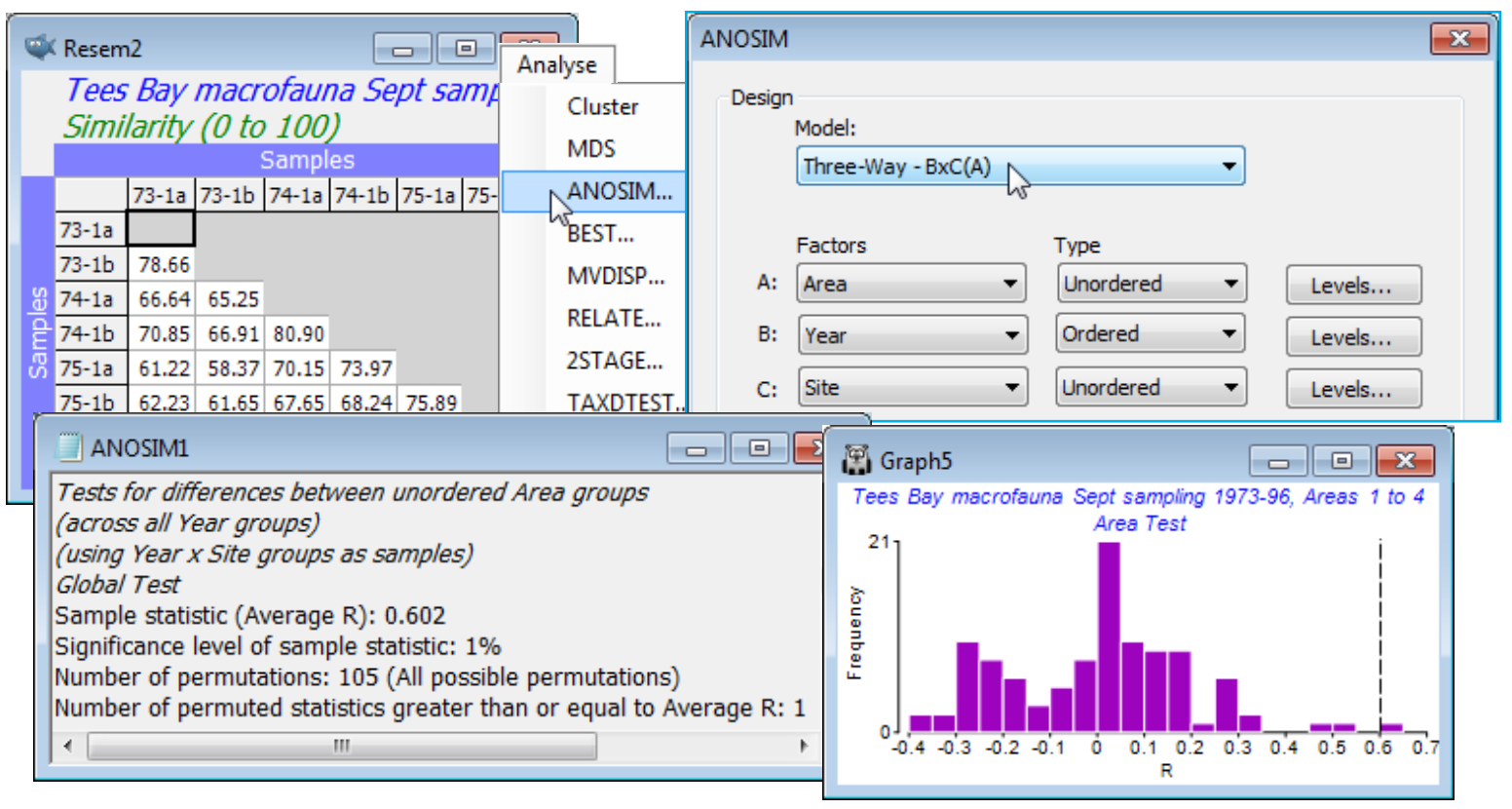
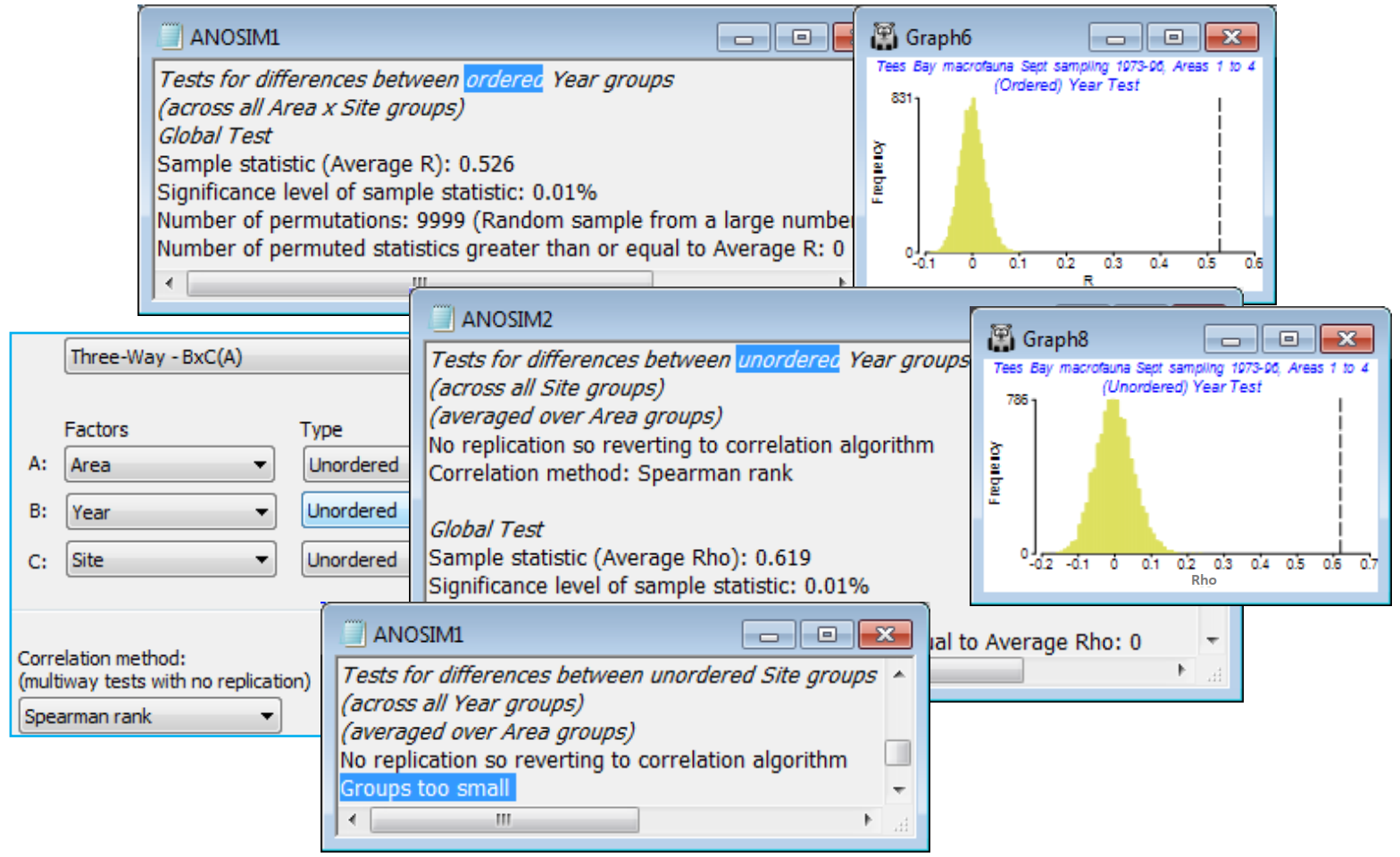
On 4th-root transformed data with Bray-Curtis similarities, Analyse>ANOSIM>(Model: Three-Way - BxC(A))>(Factors A: Area) & (B: Year) & (C: Site), with B Ordered, and then repeat the run with B Unordered, so the correlation method is needed: (Correlation method: Spearman rank).
The (unordered) Area test has average R of 0.602 and this is the most extreme value in the 105 permutations (p<1%) – the permutation procedure here, a novel one for PRIMER, permutes the site labels within the areas but carries the full set of years with it, intact, reflecting the fact that the same sites are returned to each year, rather than randomly selecting two sites from each area at each time.
The ordered Year test gives an average R$^\text{O}$ of 0.526 which the null histogram shows to be as highly significant as we wish to make it. The unordered Year test needs to use a matching statistic ($\rho$) of the year pattern over sites or areas, as indirect evidence of a time effect from its spatial conformity. The average $\rho$ of 0.619 is also very highly significant. The $\rho$ value cannot be compared with the R$^\text{O}$ statistic, though both vary in the range (roughly) 0 to (definitely) 1, but the interpretation is clear – there is a broadly consistent time pattern across the region and it is fairly strongly serial.
A test of the third factor, Site, is clearly not possible. There are no replicates below this level to utilise, so ANOSIM tries instead the indirect route of matching the among-Site pattern over the set of Years – but with only two sites per area this must fail (giving a Groups too small statement in the results window). It has been important to retain Site as a factor however (rather than regarding it as a replicate) because the same sites are returned to each year and, with this 3-way procedure, the tests for Area and Year are designed to utilise that information in a more justifiable test.
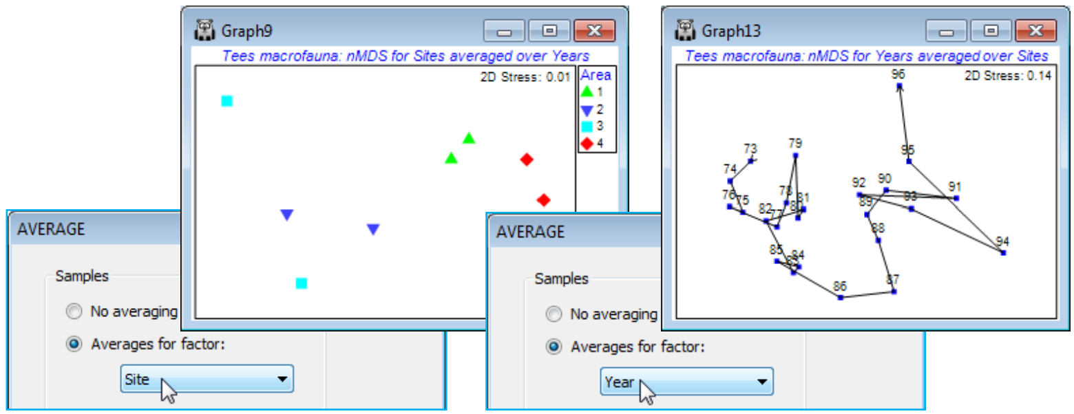
The test results again justify a summary in terms of nMDS means plots. The area effect is clearly seen in an ordination using (transformed) data averaged over the years for each site, and the time series of years, now with (transformed) data averaged over all sites, certainly indicates a strong serial change (the same time series for the 4 area levels separately is seen in Fig. 6.17 of CiMC).


