Coherent sets of abiotic variables (N Sea biomarkers)

Save the workspace as Linnhe ws, close it and re-open the data on a suite of biomarkers (‘health’ measures) from flounder sampled at five N Sea sites S3, S5, S6, S7, S9, with 10 replicate samples (pools of fish) from each site. The workspace N Sea ws in C:\Examples v7\N Sea biomarkers holds the datasheet N Sea flounder biomarkers, which was last used in Section 9 to establish differences amongst sites in the full suite of the 11 biomarkers. Two of the variables (EROD and LIPID VAC) were square-root transformed with Pre-treatment>Transformation(individual) and the full set (rename them Transformed biomarkers) then normalised to a common scale with mean 0, variance 1 (named Normalised biomarkers). It of interest here to test whether there are coherent biomarker sets – those within a set having the same pattern of response across the samples, and among sets having statistically distinguishable outcomes – and to create line plots of those common responses on the normalised scales. Here, the measurements are all matched to the individual replicates, so it is multivariate response patterns across 50 samples (not just a mean response at each of five sites) which is used to correlate the 11 variables. And it is correlation which, for most abiotic variables, is the relevant measure of variable resemblance (see Section 5). This will be Pearson correlation here, though the non-parametric Spearman correlation can be used instead.

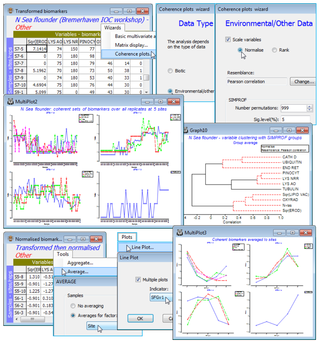
Running Wizards>Coherence plots on the active matrix Transformed biomarkers, the routine notes that the data type is defined as Other and asks for confirmation that you would like to treat these as environmental rather than community-type variables (i.e. for which correlation measures rather than the index of association are relevant). It is important to retain the ((✓Scale variables) default option, with (•Normalise) if the (Resemblance: Pearson correlation) option is chosen, even though the Pearson coefficient itself includes a normalising step. This is because the permutation process for the Type 3 SIMPROF test exchanges values across variables, within samples, prior to calculating the resemblance, and this makes no sense if the variables do not have the same scale. Of course, an alternative is to enter Wizards>Coherence plots from the Normalised biomarkers sheet, with the ((✓Scale variables) step not then required. [If you do this and still take ((✓Scale variables), PRIMER will remind you of the fact, but this is only a warning because normalising for a second time changes nothing. Similarly, if you start from Transformed biomarkers and propose to use Spearman correlation then you must take ((✓Scale variables•Rank) and (Resemblance: Change)> (Measure•Other)>((✓Correlation>Spearman rank correlation). Without the initial ranking, permut-ation of variables again makes no sense and, much more subtly, do not be lulled into thinking that Pearson correlation will then give you Spearman (since Spearman is just Pearson correlation on ranks), because after permuting ranks over variables, independently for each sample, the ranks no longer add to a constant and the re-ranking implicit in calculating Spearman becomes important].

Do not despair at this point! If you take Wizards>Coherence plots and the default (•Normalise) and (Resemblance: Pearson correlation) very little can go wrong – that is the point of a Wizard! It is only if you recreate the individual Wizard stages that you must not forget the Pre-treatment>Normalise variables step before Analyse>Resemblance>(Measure•Other>Pearson correlation) & (Analyse between•Variables), then Analyse>Cluster>CLUSTER>((✓SIMPROF test), taking the default SIMPROF dialog options, and creating (Add indicator named: SFGv1). Look at the cluster dendrogram – whether produced directly or more likely from the Wizard run – and you will see that clustering handles a correlation matrix with negative values. It is not necessary to input only (dis)similarities in (0,100) or distances over (0,) to clustering – the dendrogram y axis scale can include positive and negative correlations. However, large negative correlations between variables are treated as very low similarity, with only large positive correlations implying high similarity. This may not always be the required behaviour – indeed for these data Somerfield & Clarke (2013) make the case that knowledge of whether a biomarker increases or decreases on impact should be used to reverse some of them, by Pre-treatment>Transform(individual)>(Expression: -V), after any other transformation, so that all are expected to decline on impact. (If the behaviour on impact is not monotonic, the index may not be that useful!). That all measurements for those variables are now negative is not important since normalising restores them to the usual range of approximately (-3, 3). The coherent sets may look very different since previous opposite patterns may now match.

The main output automatically from the Wizard – or on the Normalised biomarkers running Plots>Line Plot>((✓Multiple plots>Indicator: SFGv1) – is three coherent sets and one singleton. Having used the replicates to determine the variable groupings, a neater summary is given by a means plot: Tools>Average>(Averages for factor: Site) on Normalised biomarkers, and redo the Line Plot. Save the N Sea ws workspace and close it – it will be needed at the end of the section for SIMPER.